Chapter 19 Week14: Lavaan Lab 16 Latent Growth Models
In this lab, we will:
- run and interpret a series of growth models (no growth, linear, quadratic, latent basis, spline growth);
- compare nested models and identify the best possible shape for characterizing the growth patterns;
- add predictors for the growth factors;
- run growth models on latent variables.
Load up the lavaan library:
library(lavaan)We will also need ggplot2, semPlot, and semTools. Install them if you haven’t:
#install.packages("ggplot2")
#install.packages("semPlot")
#install.packages("semTools")
library(ggplot2)
library(semPlot)
library(semTools)- For this lab, we will work with a simulated dataset # based on an example from McCoach & Kaniskan (2010).
- The main DV is Oral Reading Fluency (ORF) and is measured over 4 time points (Fall and Spring, 2 consecutive years)
- N = 277 Elementary students.
- Let’s read in the dataset:
orf <- read.csv("readingSimData.csv", header = T)Take a look at the dataset:
head(orf)## id treatmentDummy orf1 orf2 orf3 orf4
## 1 1 0 133.93092 157.81992 178.74260 151.28058
## 2 2 0 191.84038 185.91922 192.02037 175.53109
## 3 3 1 144.80922 189.83059 201.97789 218.63097
## 4 4 0 22.58577 60.99331 63.06560 56.76576
## 5 5 0 46.27449 60.32287 35.20089 65.97300
## 6 6 0 166.39739 194.00734 166.40298 169.77082sample size:
n <- nrow(orf)
n #277, just like the McCoach paper.
## [1] 277sample means and cov matrix
orfNames <- paste0("orf", 1:4)
(samMeans <- round(apply(orf[,orfNames], 2, mean), 3))
## orf1 orf2 orf3 orf4
## 108.651 134.685 136.560 163.744(samCov <- round(cov(orf[,orfNames])*((n-1)/n), 3))## orf1 orf2 orf3 orf4
## orf1 1989.243 1680.066 1718.200 1758.556
## orf2 1680.066 1817.077 1769.452 1823.106
## orf3 1718.200 1769.452 2157.290 2118.046
## orf4 1758.556 1823.106 2118.046 2525.28519.1 PART I: Spaghetti Plot
For more details, check out https://www.r-bloggers.com/my-commonly-done-ggplot2-graphs/
First, let’s use reshape() to convert wide format to long format for plotting:
growthDataLong <- reshape(orf, varying = paste0("orf", 1:4), sep = "", direction = "long")
head(growthDataLong)
## id treatmentDummy time orf
## 1.1 1 0 1 133.93092
## 2.1 2 0 1 191.84038
## 3.1 3 1 1 144.80922
## 4.1 4 0 1 22.58577
## 5.1 5 0 1 46.27449
## 6.1 6 0 1 166.39739Plot trajectory of individual with id=1
tspag_id1 = ggplot(growthDataLong[growthDataLong$id==1, ], aes(x=time, y=orf)) +
  geom_line() +
  xlab("Observation Time Point") +
  ylab("Y") +
  ylim(-40, 300) +
  ggtitle("Spaghetti plot") +
  aes(colour = factor(id))
tspag_id1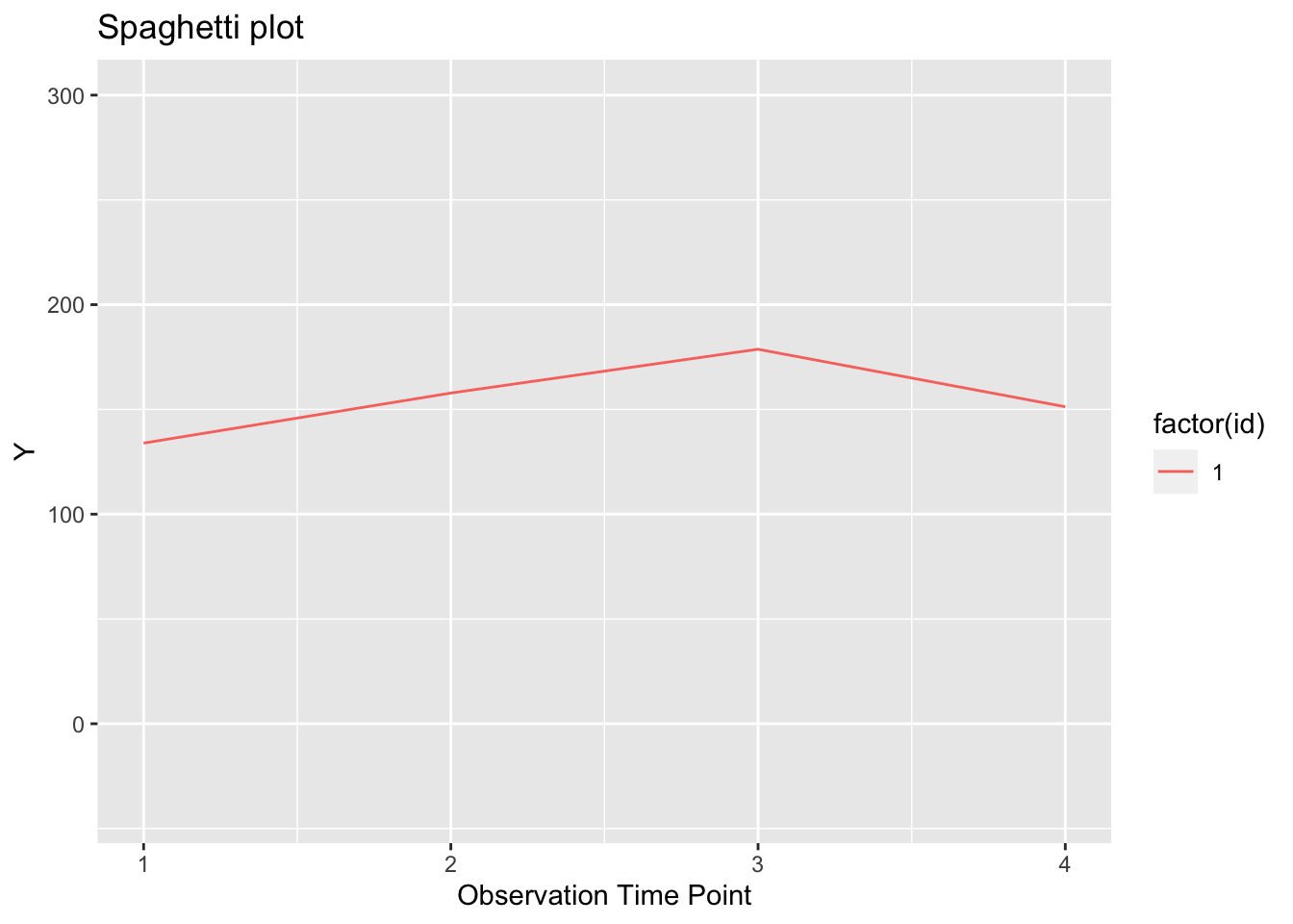
plot trajectory of everyone
tspag = ggplot(growthDataLong, aes(x=time, y=orf)) +
  geom_line(show.legend = FALSE) +
  xlab("Observation Time Point") +
  ylab("Y") +
  ylim(-40, 300) +
  ggtitle("Spaghetti plot") +
  aes(colour = factor(id))
tspag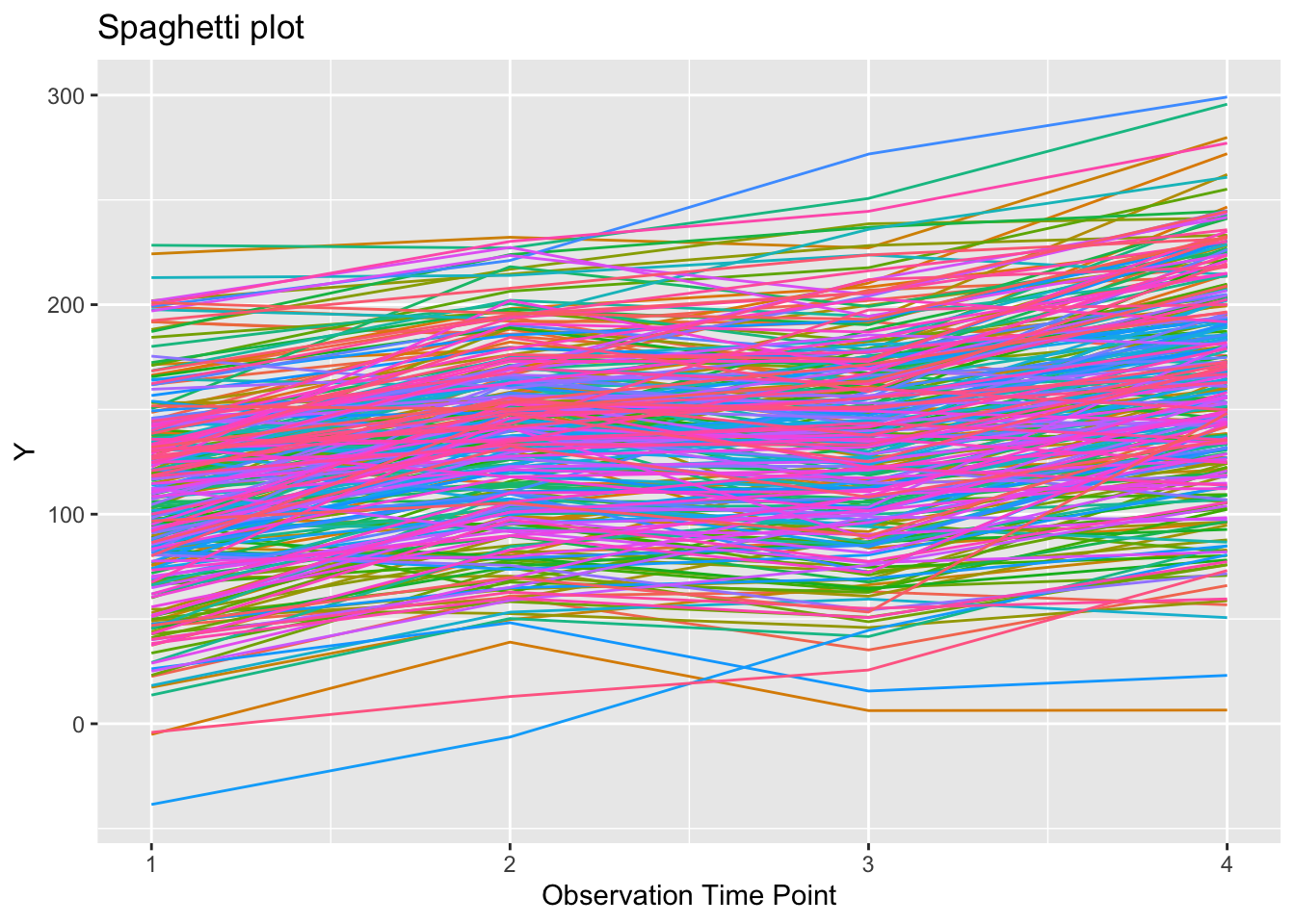
19.2 PART II: Growth Models
19.2.1 1. No growth model
- Let’s start by examining the hypothesis of no growth (intercept only)
- Intercept loads on all variables with fixed loadings of 1.0
- Use a*VAR1 to fix the coefficient of VAR1 at a:
noGrowthSyn <- "
    #Specify Latent Intercept
    I =~ 1*orf1 + 1*orf2 + 1*orf3 + 1*orf4
"
noGrowthFit <- growth(noGrowthSyn, data = orf, fixed.x = FALSE)
summary(noGrowthFit, fit.measures = T)## lavaan 0.6-12 ended normally after 80 iterations
##
## Estimator ML
## Optimization method NLMINB
## Number of model parameters 6
##
## Number of observations 277
##
## Model Test User Model:
##
## Test statistic 622.276
## Degrees of freedom 8
## P-value (Chi-square) 0.000
##
## Model Test Baseline Model:
##
## Test statistic 1367.967
## Degrees of freedom 6
## P-value 0.000
##
## User Model versus Baseline Model:
##
## Comparative Fit Index (CFI) 0.549
## Tucker-Lewis Index (TLI) 0.662
##
## Loglikelihood and Information Criteria:
##
## Loglikelihood user model (H0) -5438.991
## Loglikelihood unrestricted model (H1) -5127.853
##
## Akaike (AIC) 10889.982
## Bayesian (BIC) 10911.726
## Sample-size adjusted Bayesian (BIC) 10892.701
##
## Root Mean Square Error of Approximation:
##
## RMSEA 0.526
## 90 Percent confidence interval - lower 0.492
## 90 Percent confidence interval - upper 0.562
## P-value RMSEA <= 0.05 0.000
##
## Standardized Root Mean Square Residual:
##
## SRMR 0.263
##
## Parameter Estimates:
##
## Standard errors Standard
## Information Expected
## Information saturated (h1) model Structured
##
## Latent Variables:
## Estimate Std.Err z-value P(>|z|)
## I =~
## orf1 1.000
## orf2 1.000
## orf3 1.000
## orf4 1.000
##
## Intercepts:
## Estimate Std.Err z-value P(>|z|)
## .orf1 0.000
## .orf2 0.000
## .orf3 0.000
## .orf4 0.000
## I 134.926 2.559 52.728 0.000
##
## Variances:
## Estimate Std.Err z-value P(>|z|)
## .orf1 1132.232 102.816 11.012 0.000
## .orf2 98.891 28.254 3.500 0.000
## .orf3 312.013 38.482 8.108 0.000
## .orf4 1412.090 126.348 11.176 0.000
## I 1746.714 154.599 11.298 0.000semPaths(noGrowthFit, what='est', fade= F)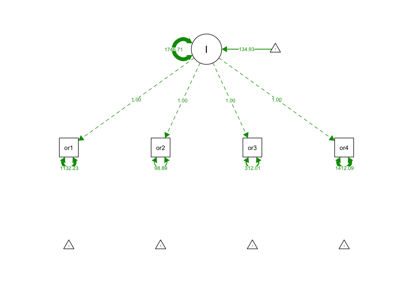
19.2.2 2. Linear growth model
- Intercept loads on all variables with fixed loadings of 1.0
- Slope loads on all variables with fixed loadings of t = 0, 1, 2, …, t-1
- t must start from 0
linearGrowthSyn <- "
    #Specify Latent Intercept and Slope
    I =~ 1*orf1 + 1*orf2 + 1*orf3 + 1*orf4
    S =~ 0*orf1 + 1*orf2 + 2*orf3 + 3*orf4
"
linearGrowthFit <- growth(linearGrowthSyn, data = orf, fixed.x = FALSE)
summary(linearGrowthFit, fit.measures = T)## lavaan 0.6-12 ended normally after 161 iterations
##
## Estimator ML
## Optimization method NLMINB
## Number of model parameters 9
##
## Number of observations 277
##
## Model Test User Model:
##
## Test statistic 159.802
## Degrees of freedom 5
## P-value (Chi-square) 0.000
##
## Model Test Baseline Model:
##
## Test statistic 1367.967
## Degrees of freedom 6
## P-value 0.000
##
## User Model versus Baseline Model:
##
## Comparative Fit Index (CFI) 0.886
## Tucker-Lewis Index (TLI) 0.864
##
## Loglikelihood and Information Criteria:
##
## Loglikelihood user model (H0) -5207.754
## Loglikelihood unrestricted model (H1) -5127.853
##
## Akaike (AIC) 10433.508
## Bayesian (BIC) 10466.124
## Sample-size adjusted Bayesian (BIC) 10437.586
##
## Root Mean Square Error of Approximation:
##
## RMSEA 0.334
## 90 Percent confidence interval - lower 0.291
## 90 Percent confidence interval - upper 0.380
## P-value RMSEA <= 0.05 0.000
##
## Standardized Root Mean Square Residual:
##
## SRMR 0.076
##
## Parameter Estimates:
##
## Standard errors Standard
## Information Expected
## Information saturated (h1) model Structured
##
## Latent Variables:
## Estimate Std.Err z-value P(>|z|)
## I =~
## orf1 1.000
## orf2 1.000
## orf3 1.000
## orf4 1.000
## S =~
## orf1 0.000
## orf2 1.000
## orf3 2.000
## orf4 3.000
##
## Covariances:
## Estimate Std.Err z-value P(>|z|)
## I ~~
## S -4.269 29.309 -0.146 0.884
##
## Intercepts:
## Estimate Std.Err z-value P(>|z|)
## .orf1 0.000
## .orf2 0.000
## .orf3 0.000
## .orf4 0.000
## I 110.504 2.585 42.746 0.000
## S 17.218 0.628 27.410 0.000
##
## Variances:
## Estimate Std.Err z-value P(>|z|)
## .orf1 210.000 45.503 4.615 0.000
## .orf2 257.156 30.447 8.446 0.000
## .orf3 302.851 34.737 8.718 0.000
## .orf4 168.261 48.428 3.474 0.001
## I 1698.098 159.067 10.675 0.000
## S 70.482 11.729 6.009 0.000semPaths(linearGrowthFit, what='est', fade= F)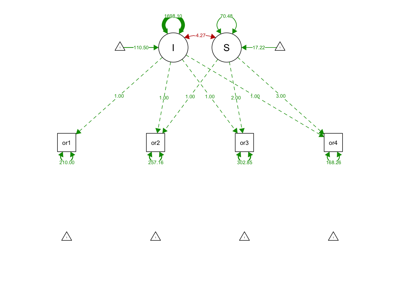
19.2.3 3. Quadratic growth model
- Intercept loads on all variables with fixed loadings of 1.0
- Slope loads on all variables with fixed loadings of t = 0, 1, 2, …, t-1
- Quadratic loads on all variables with fixed loadings of t^2 = 0, 1, 4, …, (t-1)^2
- Quadratic has no variance and covariances
quadGrowthSyn <- "
    #int and slope factors
    I =~ 1*orf1 + 1*orf2 + 1*orf3 + 1*orf4
    S =~ 0*orf1 + 1*orf2 + 2*orf3 + 3*orf4
    #quadratic factor = slope^2
    quadS =~ 0*orf1 + 1*orf2 + 4*orf3 + 9*orf4
"
quadGrowthFit <- growth(quadGrowthSyn, data = orf, fixed.x = FALSE)## Warning in lav_object_post_check(object): lavaan WARNING: some
## estimated ov variances are negative## Warning in lav_object_post_check(object): lavaan WARNING: some
## estimated lv variances are negativeIf you get the following warning messages:
1: In lav_object_post_check(object) : lavaan WARNING: some estimated ov variances are negative
- Use var1~~0*var2 to fix the (co)variances at 0
quadGrowthSyn_noQuad <- "
    #int and slope factors
    I =~ 1*orf1 + 1*orf2 + 1*orf3 + 1*orf4
    S =~ 0*orf1 + 1*orf2 + 2*orf3 + 3*orf4
    #quadratic factor = slope^2
    quadS =~ 0*orf1 + 1*orf2 + 4*orf3 + 9*orf4

    quadS ~~ 0*quadS #restrict quadratic variance to 0
    quadS ~~ 0*I #restrict quadratic covariance with I to 0
    quadS ~~ 0*S #restrict quadratic covariance with S to 0
"
quadGrowthNoquadFit <- growth(quadGrowthSyn_noQuad,
data = orf, fixed.x = FALSE)
summary(quadGrowthNoquadFit, fit.measures = T)## lavaan 0.6-12 ended normally after 166 iterations
##
## Estimator ML
## Optimization method NLMINB
## Number of model parameters 10
##
## Number of observations 277
##
## Model Test User Model:
##
## Test statistic 159.759
## Degrees of freedom 4
## P-value (Chi-square) 0.000
##
## Model Test Baseline Model:
##
## Test statistic 1367.967
## Degrees of freedom 6
## P-value 0.000
##
## User Model versus Baseline Model:
##
## Comparative Fit Index (CFI) 0.886
## Tucker-Lewis Index (TLI) 0.828
##
## Loglikelihood and Information Criteria:
##
## Loglikelihood user model (H0) -5207.733
## Loglikelihood unrestricted model (H1) -5127.853
##
## Akaike (AIC) 10435.465
## Bayesian (BIC) 10471.705
## Sample-size adjusted Bayesian (BIC) 10439.997
##
## Root Mean Square Error of Approximation:
##
## RMSEA 0.375
## 90 Percent confidence interval - lower 0.326
## 90 Percent confidence interval - upper 0.426
## P-value RMSEA <= 0.05 0.000
##
## Standardized Root Mean Square Residual:
##
## SRMR 0.077
##
## Parameter Estimates:
##
## Standard errors Standard
## Information Expected
## Information saturated (h1) model Structured
##
## Latent Variables:
## Estimate Std.Err z-value P(>|z|)
## I =~
## orf1 1.000
## orf2 1.000
## orf3 1.000
## orf4 1.000
## S =~
## orf1 0.000
## orf2 1.000
## orf3 2.000
## orf4 3.000
## quadS =~
## orf1 0.000
## orf2 1.000
## orf3 4.000
## orf4 9.000
##
## Covariances:
## Estimate Std.Err z-value P(>|z|)
## I ~~
## quadS 0.000
## S ~~
## quadS 0.000
## I ~~
## S -4.082 29.338 -0.139 0.889
##
## Intercepts:
## Estimate Std.Err z-value P(>|z|)
## .orf1 0.000
## .orf2 0.000
## .orf3 0.000
## .orf4 0.000
## I 110.574 2.619 42.216 0.000
## S 16.827 1.544 10.897 0.000
## quadS 0.129 0.460 0.281 0.779
##
## Variances:
## Estimate Std.Err z-value P(>|z|)
## quadS 0.000
## .orf1 210.600 45.691 4.609 0.000
## .orf2 261.091 30.735 8.495 0.000
## .orf3 298.679 34.435 8.674 0.000
## .orf4 167.168 48.238 3.465 0.001
## I 1697.894 159.144 10.669 0.000
## S 70.527 11.730 6.013 0.000semPaths(quadGrowthNoquadFit, what='est', fade= F)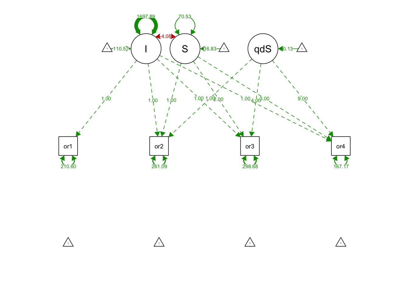
19.2.4 4. Latent basis growth model (extension of linear growth model)
- Intercept loads on all variables with fixed loadings of 1.0
- Slope loads on all variables with free loadings between 0 and t-1
latentBasisSyn <- "
    #Int and slope specification
    I =~ 1*orf1 + 1*orf2 + 1*orf3 + 1*orf4

    #orf2 and orf3 are free in the latent basis specification
    S =~ 0*orf1 + alpha1*orf2 + alpha2*orf3 + 3*orf4
"
latentBasisFit <- growth(latentBasisSyn,
data = orf,
fixed.x = FALSE)
summary(latentBasisFit, fit.measures = T)## lavaan 0.6-12 ended normally after 171 iterations
##
## Estimator ML
## Optimization method NLMINB
## Number of model parameters 11
##
## Number of observations 277
##
## Model Test User Model:
##
## Test statistic 41.591
## Degrees of freedom 3
## P-value (Chi-square) 0.000
##
## Model Test Baseline Model:
##
## Test statistic 1367.967
## Degrees of freedom 6
## P-value 0.000
##
## User Model versus Baseline Model:
##
## Comparative Fit Index (CFI) 0.972
## Tucker-Lewis Index (TLI) 0.943
##
## Loglikelihood and Information Criteria:
##
## Loglikelihood user model (H0) -5148.648
## Loglikelihood unrestricted model (H1) -5127.853
##
## Akaike (AIC) 10319.297
## Bayesian (BIC) 10359.161
## Sample-size adjusted Bayesian (BIC) 10324.281
##
## Root Mean Square Error of Approximation:
##
## RMSEA 0.215
## 90 Percent confidence interval - lower 0.160
## 90 Percent confidence interval - upper 0.276
## P-value RMSEA <= 0.05 0.000
##
## Standardized Root Mean Square Residual:
##
## SRMR 0.042
##
## Parameter Estimates:
##
## Standard errors Standard
## Information Expected
## Information saturated (h1) model Structured
##
## Latent Variables:
## Estimate Std.Err z-value P(>|z|)
## I =~
## orf1 1.000
## orf2 1.000
## orf3 1.000
## orf4 1.000
## S =~
## orf1 0.000
## orf2 (alp1) 1.343 0.056 23.780 0.000
## orf3 (alp2) 1.575 0.058 27.342 0.000
## orf4 3.000
##
## Covariances:
## Estimate Std.Err z-value P(>|z|)
## I ~~
## S -1.364 30.564 -0.045 0.964
##
## Intercepts:
## Estimate Std.Err z-value P(>|z|)
## .orf1 0.000
## .orf2 0.000
## .orf3 0.000
## .orf4 0.000
## I 108.867 2.633 41.354 0.000
## S 18.294 0.644 28.418 0.000
##
## Variances:
## Estimate Std.Err z-value P(>|z|)
## .orf1 232.136 45.754 5.074 0.000
## .orf2 200.709 24.071 8.338 0.000
## .orf3 215.666 25.245 8.543 0.000
## .orf4 193.173 49.612 3.894 0.000
## I 1688.626 159.099 10.614 0.000
## S 67.573 12.843 5.261 0.000semPaths(latentBasisFit, what='est', fade= F)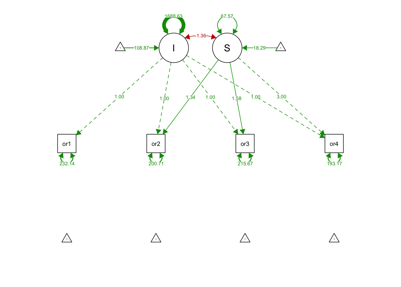
RMSEA failed us… one approach is to use model modification indices:
modindices(latentBasisFit,sort. = T)## lhs op rhs mi epc sepc.lv sepc.all sepc.nox
## 27 orf3 ~~ orf4 37.677 285.256 285.256 1.398 1.398
## 17 orf2 ~1 37.648 21.985 21.985 0.491 0.491
## 18 orf3 ~1 29.423 -20.326 -20.326 -0.447 -0.447
## 26 orf2 ~~ orf4 29.372 -191.644 -191.644 -0.973 -0.973
## 24 orf1 ~~ orf4 27.665 701.390 701.390 3.312 3.312
## 22 orf1 ~~ orf2 17.100 164.959 164.959 0.764 0.764
## 23 orf1 ~~ orf3 13.434 -113.046 -113.046 -0.505 -0.505
## 16 orf1 ~1 12.388 -47.985 -47.985 -1.095 -1.095
## 3 I =~ orf3 10.891 -0.077 -3.175 -0.070 -0.070
## 2 I =~ orf2 5.875 0.060 2.461 0.055 0.055
## 4 I =~ orf4 4.587 0.152 6.261 0.126 0.126
## 1 I =~ orf1 0.801 0.063 2.577 0.059 0.059
## 25 orf2 ~~ orf3 0.014 -4.660 -4.660 -0.022 -0.022
## 19 orf4 ~1 0.010 -1.524 -1.524 -0.031 -0.031Another approach is to use Spline Growth Model.
19.2.5 5. Spline Growth Model
splineGrowthSyn <- "
    #Specify Latent Intercept and Slope
    I =~ 1*orf1 + 1*orf2 + 1*orf3 + 1*orf4
    S =~ 0*orf1 + 1*orf2 + 2*orf3 + 3*orf4

    #summer is the spline variable
    summer =~ 0*orf1 + 0*orf2 + 1*orf3 + 1*orf4

    #Summer gets a mean but no variance
    summer ~ 1
    summer ~~ 0*summer

    #Summer is uncorrelated with I and S
    summer ~~ 0*I
    summer ~~ 0*S
"
splineGrowthFit <- growth(splineGrowthSyn, data = orf, fixed.x = FALSE)
summary(splineGrowthFit, fit.measures = T)## lavaan 0.6-12 ended normally after 165 iterations
##
## Estimator ML
## Optimization method NLMINB
## Number of model parameters 10
##
## Number of observations 277
##
## Model Test User Model:
##
## Test statistic 8.029
## Degrees of freedom 4
## P-value (Chi-square) 0.091
##
## Model Test Baseline Model:
##
## Test statistic 1367.967
## Degrees of freedom 6
## P-value 0.000
##
## User Model versus Baseline Model:
##
## Comparative Fit Index (CFI) 0.997
## Tucker-Lewis Index (TLI) 0.996
##
## Loglikelihood and Information Criteria:
##
## Loglikelihood user model (H0) -5131.868
## Loglikelihood unrestricted model (H1) -5127.853
##
## Akaike (AIC) 10283.735
## Bayesian (BIC) 10319.975
## Sample-size adjusted Bayesian (BIC) 10288.267
##
## Root Mean Square Error of Approximation:
##
## RMSEA 0.060
## 90 Percent confidence interval - lower 0.000
## 90 Percent confidence interval - upper 0.121
## P-value RMSEA <= 0.05 0.320
##
## Standardized Root Mean Square Residual:
##
## SRMR 0.023
##
## Parameter Estimates:
##
## Standard errors Standard
## Information Expected
## Information saturated (h1) model Structured
##
## Latent Variables:
## Estimate Std.Err z-value P(>|z|)
## I =~
## orf1 1.000
## orf2 1.000
## orf3 1.000
## orf4 1.000
## S =~
## orf1 0.000
## orf2 1.000
## orf3 2.000
## orf4 3.000
## summer =~
## orf1 0.000
## orf2 0.000
## orf3 1.000
## orf4 1.000
##
## Covariances:
## Estimate Std.Err z-value P(>|z|)
## I ~~
## summer 0.000
## S ~~
## summer 0.000
## I ~~
## S 3.511 28.391 0.124 0.902
##
## Intercepts:
## Estimate Std.Err z-value P(>|z|)
## summer -24.715 1.804 -13.697 0.000
## .orf1 0.000
## .orf2 0.000
## .orf3 0.000
## .orf4 0.000
## I 108.303 2.579 41.998 0.000
## S 26.616 0.986 26.987 0.000
##
## Variances:
## Estimate Std.Err z-value P(>|z|)
## summer 0.000
## .orf1 246.662 40.796 6.046 0.000
## .orf2 165.717 21.986 7.537 0.000
## .orf3 183.428 23.958 7.656 0.000
## .orf4 219.241 42.313 5.181 0.000
## I 1670.038 155.803 10.719 0.000
## S 65.687 10.741 6.116 0.000semPaths(splineGrowthFit, what='est', fade= F)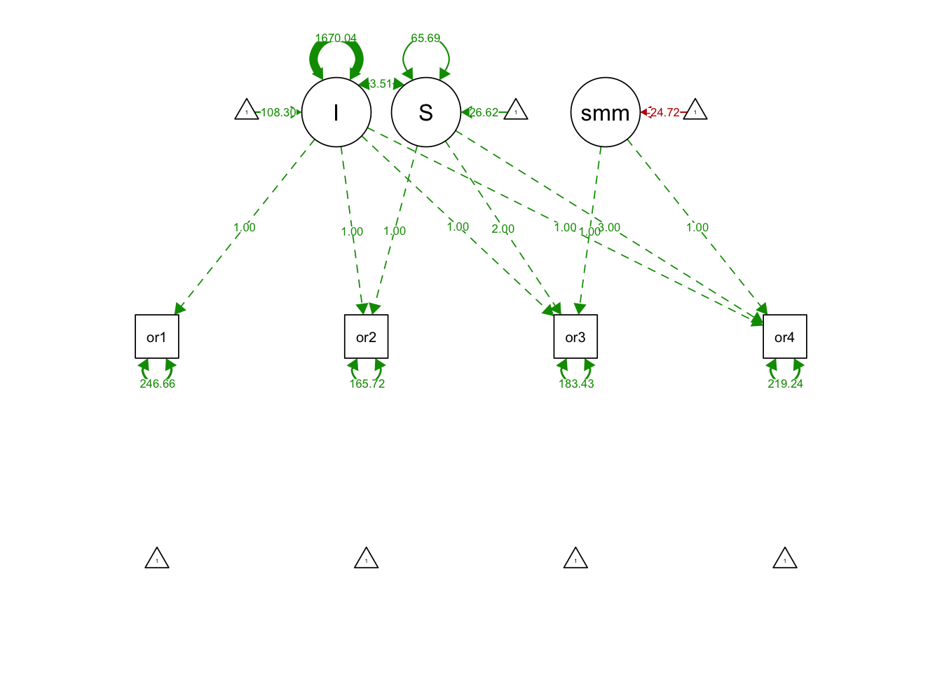
19.2.6 Model Comparison
lavTestLRT(noGrowthFit, linearGrowthFit)## Chi-Squared Difference Test
##
## Df AIC BIC Chisq Chisq diff Df diff Pr(>Chisq)
## linearGrowthFit 5 10434 10466 159.80
## noGrowthFit 8 10890 10912 622.28 462.47 3 < 2.2e-16
##
## linearGrowthFit
## noGrowthFit ***
## ---
## Signif. codes: 0 '***' 0.001 '**' 0.01 '*' 0.05 '.' 0.1 ' ' 1- Linear Growth Model fits significantly better than No Growth Model
lavTestLRT(linearGrowthFit, quadGrowthNoquadFit)## Chi-Squared Difference Test
##
## Df AIC BIC Chisq Chisq diff Df diff
## quadGrowthNoquadFit 4 10436 10472 159.76
## linearGrowthFit 5 10434 10466 159.80 0.042546 1
## Pr(>Chisq)
## quadGrowthNoquadFit
## linearGrowthFit 0.8366- Linear Growth Model fits almost the same as the Quadratic Growth Model (keep linear model due to parsimony principle)
lavTestLRT(linearGrowthFit, latentBasisFit)## Chi-Squared Difference Test
##
## Df AIC BIC Chisq Chisq diff Df diff Pr(>Chisq)
## latentBasisFit 3 10319 10359 41.591
## linearGrowthFit 5 10434 10466 159.802 118.21 2 < 2.2e-16
##
## latentBasisFit
## linearGrowthFit ***
## ---
## Signif. codes: 0 '***' 0.001 '**' 0.01 '*' 0.05 '.' 0.1 ' ' 1- Latent Basis Model fits significantly better than Linear Growth Model
lavTestLRT(linearGrowthFit, splineGrowthFit)## Chi-Squared Difference Test
##
## Df AIC BIC Chisq Chisq diff Df diff Pr(>Chisq)
## splineGrowthFit 4 10284 10320 8.0292
## linearGrowthFit 5 10434 10466 159.8018 151.77 1 < 2.2e-16
##
## splineGrowthFit
## linearGrowthFit ***
## ---
## Signif. codes: 0 '***' 0.001 '**' 0.01 '*' 0.05 '.' 0.1 ' ' 1- Spline Growth Model also fits significantly better than Linear Growth Model
19.2.7 6. Final Model: Spline Growth Model with a binary treatment predictor
splineGrowthTreatmentPredictorSyn <- "
    #Specify Latent Intercept and Slope
    I =~ 1*orf1 + 1*orf2 + 1*orf3 + 1*orf4
    S =~ 0*orf1 + 1*orf2 + 2*orf3 + 3*orf4

    #summer is the spline variable
    summer =~ 0*orf1 + 0*orf2 + 1*orf3 + 1*orf4

    #Summer gets a mean but no variance
    summer ~~ 0*summer

    #Summer is uncorrelated with I and S
    summer ~~ 0*I
    summer ~~ 0*S

    #Intercept, Slope, and Summer regressed on (predicted by) treatment
    I ~ treatmentDummy
    S ~ treatmentDummy
    summer ~ treatmentDummy
"- When including external predictors, we need to turn on fixed.x = T…
- otherwise you’ll get a warning message and misleading model fit:
# do not do this:
splineGrowthTreatPredictorFit <- growth(splineGrowthTreatmentPredictorSyn,
                                       data = orf,
                                       fixed.x = F) # <- Here
## Warning in lav_data_full(data = data, group = group, cluster =
## cluster, : lavaan WARNING: some observed variances are (at least) a
## factor 1000 times larger than others; use varTable(fit) to investigate## Warning in lav_partable_check(lavpartable, categorical = lavoptions$.categorical, : lavaan WARNING: automatically added intercepts are set to zero:
## [treatmentDummy]Instead, turn on fixed.x = T:
splineGrowthTreatPredictorFit <- growth(splineGrowthTreatmentPredictorSyn,
                                       data = orf,
                                       fixed.x = T) # <- Here
summary(splineGrowthTreatPredictorFit, fit.measures = T)
## lavaan 0.6-12 ended normally after 213 iterations
##
## Estimator ML
## Optimization method NLMINB
## Number of model parameters 13
##
## Number of observations 277
##
## Model Test User Model:
##
## Test statistic 8.288
## Degrees of freedom 5
## P-value (Chi-square) 0.141
##
## Model Test Baseline Model:
##
## Test statistic 1604.488
## Degrees of freedom 10
## P-value 0.000
##
## User Model versus Baseline Model:
##
## Comparative Fit Index (CFI) 0.998
## Tucker-Lewis Index (TLI) 0.996
##
## Loglikelihood and Information Criteria:
##
## Loglikelihood user model (H0) -5013.737
## Loglikelihood unrestricted model (H1) -5009.593
##
## Akaike (AIC) 10053.473
## Bayesian (BIC) 10100.585
## Sample-size adjusted Bayesian (BIC) 10059.364
##
## Root Mean Square Error of Approximation:
##
## RMSEA 0.049
## 90 Percent confidence interval - lower 0.000
## 90 Percent confidence interval - upper 0.105
## P-value RMSEA <= 0.05 0.443
##
## Standardized Root Mean Square Residual:
##
## SRMR 0.019
##
## Parameter Estimates:
##
## Standard errors Standard
## Information Expected
## Information saturated (h1) model Structured
##
## Latent Variables:
## Estimate Std.Err z-value P(>|z|)
## I =~
## orf1 1.000
## orf2 1.000
## orf3 1.000
## orf4 1.000
## S =~
## orf1 0.000
## orf2 1.000
## orf3 2.000
## orf4 3.000
## summer =~
## orf1 0.000
## orf2 0.000
## orf3 1.000
## orf4 1.000
##
## Regressions:
## Estimate Std.Err z-value P(>|z|)
## I ~
## treatmentDummy 1.181 5.165 0.229 0.819
## S ~
## treatmentDummy 14.530 1.725 8.425 0.000
## summer ~
## treatmentDummy 2.874 3.650 0.787 0.431
##
## Covariances:
## Estimate Std.Err z-value P(>|z|)
## .I ~~
## .summer 0.000
## .S ~~
## .summer 0.000
## .I ~~
## .S -2.783 19.658 -0.142 0.887
##
## Intercepts:
## Estimate Std.Err z-value P(>|z|)
## .orf1 0.000
## .orf2 0.000
## .orf3 0.000
## .orf4 0.000
## .I 107.754 3.565 30.223 0.000
## .S 19.690 1.191 16.538 0.000
## .summer -26.082 2.520 -10.352 0.000
##
## Variances:
## Estimate Std.Err z-value P(>|z|)
## .summer 0.000
## .orf1 232.349 33.038 7.033 0.000
## .orf2 171.092 20.837 8.211 0.000
## .orf3 189.396 22.176 8.541 0.000
## .orf4 206.315 31.878 6.472 0.000
## .I 1678.278 155.946 10.762 0.000
## .S 5.773 6.112 0.944 0.345semPaths(splineGrowthTreatPredictorFit, what='est', fade= F)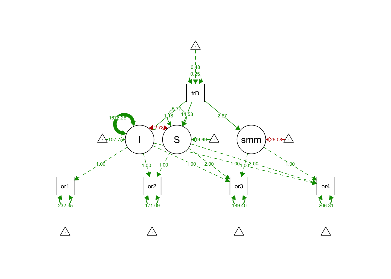
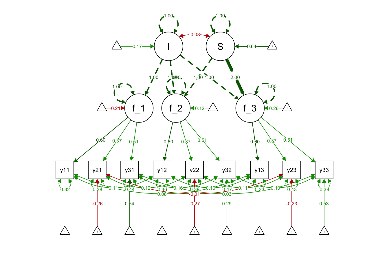
19.3 PART III: LGM on Latent Variables
19.3.1 Example
Please go over the checklist:
- Make sure the latent variables satisfy longitudinal measurement invariance at the level of scalar invariance or above
- Use the loadings over time (i.e., metric invariance)
- No need to correlate the latent factors
- Add intercepts for all indicators EXCEPT for marker indicators
- Add correlated residuals for repeated measures of the same indicators
- Use std.lv = TRUE as the scaling method in growth()
For this example, we will use the dataset exLong from package semTools:
data(exLong)
head(exLong)
## sex y1t1 y2t1 y3t1 y1t2 y2t2
## 1 female 2.7625423 2.2812510 2.49656014 2.9499400 1.12338865
## 2 female 0.2707267 -0.7830365 -0.23554656 0.4631038 0.37536412
## 3 female -0.2604141 0.3146881 1.21590069 0.3528803 0.00986991
## 4 female -1.0227953 -1.3454733 0.04899156 1.9530137 -1.03357363
## 5 female 0.7385408 -0.6027341 0.42557808 -0.2027779 -0.34937717
## 6 female 0.5864878 -0.4659974 0.10691644 0.7869085 -0.31982170
## y3t2 y1t3 y2t3 y3t3
## 1 2.1505466 1.912824 1.9625734 2.4403812
## 2 2.0283960 2.112440 0.4326280 2.6352259
## 3 1.0709696 1.472736 1.1951005 1.4287358
## 4 2.7817132 1.249376 -0.5369589 2.3371304
## 5 1.1865013 1.425101 1.8539630 2.0861627
## 6 0.4825864 -1.201912 -2.0090700 -0.8366951?exLongThe syntax for linear growth model with latent variables:
exLinearGrowthsyn <- "

  # Use the loadings over time (i.e., metric invariance)
  f_t1 =~ lamb1*y1t1 + lamb2*y2t1 + lamb3*y3t1
  f_t2 =~ lamb1*y1t2 + lamb2*y2t2 + lamb3*y3t2
  f_t3 =~ lamb1*y1t3 + lamb2*y2t3 + lamb3*y3t3

  #Int and slope specification
    I =~ 1*f_t1 + 1*f_t2 + 1*f_t3
    S =~ 0*f_t1 + 1*f_t2 + 2*f_t3

    # Add intercepts for all indicators EXCEPT for marker indicators
  y2t1 ~ 1
  y3t1 ~ 1
  y2t2 ~ 1
  y3t2 ~ 1
    y2t3 ~ 1
  y3t3 ~ 1

    # Add correlated residuals for repeated measures of the same indicators
    y1t1 ~~ y1t2
    y1t1 ~~ y1t3
    y1t2 ~~ y1t3
    y2t1 ~~ y2t2
    y2t1 ~~ y2t3
    y2t2 ~~ y2t3
    y3t1 ~~ y3t2
    y3t1 ~~ y3t3
    y3t2 ~~ y3t3
"
Use std.lv = TRUE as the scaling method in growth():
exLinearGrowthFit <- growth(exLinearGrowthsyn,
                         data = exLong,
                         fixed.x = FALSE,
                         std.lv = TRUE)
## Warning in lav_model_vcov(lavmodel = lavmodel, lavsamplestats = lavsamplestats, : lavaan WARNING:
## The variance-covariance matrix of the estimated parameters (vcov)
## does not appear to be positive definite! The smallest eigenvalue
## (= 3.760605e-18) is close to zero. This may be a symptom that the
## model is not identified.summary(exLinearGrowthFit, fit.measures = T)## lavaan 0.6-12 ended normally after 36 iterations
##
## Estimator ML
## Optimization method NLMINB
## Number of model parameters 39
## Number of equality constraints 6
##
## Number of observations 200
##
## Model Test User Model:
##
## Test statistic 72.972
## Degrees of freedom 21
## P-value (Chi-square) 0.000
##
## Model Test Baseline Model:
##
## Test statistic 1126.037
## Degrees of freedom 36
## P-value 0.000
##
## User Model versus Baseline Model:
##
## Comparative Fit Index (CFI) 0.952
## Tucker-Lewis Index (TLI) 0.918
##
## Loglikelihood and Information Criteria:
##
## Loglikelihood user model (H0) -2209.468
## Loglikelihood unrestricted model (H1) -2172.981
##
## Akaike (AIC) 4484.935
## Bayesian (BIC) 4593.780
## Sample-size adjusted Bayesian (BIC) 4489.232
##
## Root Mean Square Error of Approximation:
##
## RMSEA 0.111
## 90 Percent confidence interval - lower 0.084
## 90 Percent confidence interval - upper 0.140
## P-value RMSEA <= 0.05 0.000
##
## Standardized Root Mean Square Residual:
##
## SRMR 0.181
##
## Parameter Estimates:
##
## Standard errors Standard
## Information Expected
## Information saturated (h1) model Structured
##
## Latent Variables:
## Estimate Std.Err z-value P(>|z|)
## f_t1 =~
## y1t1 (lmb1) 0.595 0.027 22.333 0.000
## y2t1 (lmb2) 0.371 0.021 18.042 0.000
## y3t1 (lmb3) 0.513 0.025 20.776 0.000
## f_t2 =~
## y1t2 (lmb1) 0.595 0.027 22.333 0.000
## y2t2 (lmb2) 0.371 0.021 18.042 0.000
## y3t2 (lmb3) 0.513 0.025 20.776 0.000
## f_t3 =~
## y1t3 (lmb1) 0.595 0.027 22.333 0.000
## y2t3 (lmb2) 0.371 0.021 18.042 0.000
## y3t3 (lmb3) 0.513 0.025 20.776 0.000
## I =~
## f_t1 1.000
## f_t2 1.000
## f_t3 1.000
## S =~
## f_t1 0.000
## f_t2 1.000
## f_t3 2.000
##
## Covariances:
## Estimate Std.Err z-value P(>|z|)
## .y1t1 ~~
## .y1t2 0.112 0.049 2.315 0.021
## .y1t3 0.083 0.045 1.851 0.064
## .y1t2 ~~
## .y1t3 0.162 0.056 2.906 0.004
## .y2t1 ~~
## .y2t2 0.117 0.034 3.452 0.001
## .y2t3 -0.009 0.034 -0.283 0.777
## .y2t2 ~~
## .y2t3 0.114 0.036 3.134 0.002
## .y3t1 ~~
## .y3t2 0.158 0.046 3.392 0.001
## .y3t3 0.029 0.042 0.690 0.490
## .y3t2 ~~
## .y3t3 0.095 0.047 2.029 0.042
## I ~~
## S -0.079 0.119 -0.662 0.508
##
## Intercepts:
## Estimate Std.Err z-value P(>|z|)
## .y2t1 -0.264 0.050 -5.288 0.000
## .y3t1 0.540 0.058 9.269 0.000
## .y2t2 -0.266 0.057 -4.689 0.000
## .y3t2 0.291 0.068 4.287 0.000
## .y2t3 -0.228 0.064 -3.584 0.000
## .y3t3 0.534 0.071 7.542 0.000
## .y1t1 0.000
## .y1t2 0.000
## .y1t3 0.000
## .f_t1 -0.207 0.068 -3.036 0.002
## .f_t2 0.119 0.080 1.484 0.138
## .f_t3 0.262 0.050 5.201 0.000
## I 0.174 0.065 2.683 0.007
## S 0.643 0.071 9.078 0.000
##
## Variances:
## Estimate Std.Err z-value P(>|z|)
## .y1t1 0.320 0.062 5.191 0.000
## .y2t1 0.376 0.045 8.418 0.000
## .y3t1 0.440 0.060 7.277 0.000
## .y1t2 0.457 0.077 5.946 0.000
## .y2t2 0.394 0.048 8.224 0.000
## .y3t2 0.474 0.068 7.006 0.000
## .y1t3 0.333 0.077 4.305 0.000
## .y2t3 0.433 0.052 8.397 0.000
## .y3t3 0.381 0.065 5.895 0.000
## .f_t1 1.000
## .f_t2 1.000
## .f_t3 1.000
## I 1.000
## S 1.000semPaths(exLinearGrowthFit, what='est', fade= F)