Chapter 4 Lavaan Lab 2: Mediation and Indirect Effects
In this lab, we will learn how to:
- perform a simple mediation analysis using Preacher & Hayes (2004) + Bootstrap
- test mediation effects in the eating disorder path model
4.1 Reading-In and Working With Realistic Datasets In R
If your data (eatingDisorderSimData.csv) is stored in you current working directory, then simply load your data by typing the name of the .csv file:
labData <- read.csv(file = "eatingDisorderSimData.csv", header = T, sep = ",")4.2 Using Lavaan For Mediation Models - Preacher & Hayes’s
Load the package:
library(lavaan)- Part I: Writing the Model Syntax
- Part II: Analyzing the Model Using Your Dataset
- Part III: Examining the results.
4.3 PART I: # Follow the two equations of M (DietSE) & Y (Bulimia)
Diet Self-Efficacy = BMI + Disturbance
Bulimic Symptoms = BMI + Diet Self-Efficacy + Disturbance
Let’s write some model syntax:
ex1MediationSyntax <- "              #opening a quote
    #Regressions
    DietSE ~ BMI                    #M ~ X regression (a path)
    Bulimia ~ BMI + DietSE          #Y ~ X + M regression (c prime and b)
    "
No need to fix disturbance covariances in simple mediation as none was estimated
4.4 PART II Let’s run our model!
let fixed.x=FALSE to print more lines
ex1fit_freeX <- lavaan::sem(model = ex1MediationSyntax, data = labData, fixed.x = FALSE)
summary(ex1fit_freeX)
## lavaan 0.6-12 ended normally after 1 iterations
##
## Estimator ML
## Optimization method NLMINB
## Number of model parameters 6
##
## Number of observations 1339
##
## Model Test User Model:
##
## Test statistic 0.000
## Degrees of freedom 0
##
## Parameter Estimates:
##
## Standard errors Standard
## Information Expected
## Information saturated (h1) model Structured
##
## Regressions:
## Estimate Std.Err z-value P(>|z|)
## DietSE ~
## BMI -0.100 0.026 -3.861 0.000
## Bulimia ~
## BMI 0.129 0.026 4.960 0.000
## DietSE -0.213 0.028 -7.725 0.000
##
## Variances:
## Estimate Std.Err z-value P(>|z|)
## .DietSE 0.955 0.037 25.875 0.000
## .Bulimia 0.968 0.037 25.875 0.000
## BMI 1.073 0.041 25.875 0.000note that there are six parameter estimates and df = 0.
But the output does not include the mediation effect a*b?
4.4.1 Label the mediation effect
Let’s learn how to label parameters
great tutorial example: http://lavaan.ugent.be/tutorial/mediation.html
To label a parameter, include the coefficient label and an asterisk * before the variable to be labelled.
E.g., y ~ b1x + b2m
This would give x the label b1 and m the label b2 in the y regression.
ex2MediationSyntax <- "                         #opening a quote
    #Regressions
    DietSE ~ a*BMI                      #Label the a coefficient in the M regression.
    Bulimia ~ cPrime*BMI + b*DietSE   #Label the direct effect (cPrime) of X and direct effect of M (b) in the Y regression.
    "
What does this do?
ex2fit <- lavaan::sem(model = ex2MediationSyntax, data = labData, fixed.x=FALSE)
summary(ex2fit)
## lavaan 0.6-12 ended normally after 1 iterations
##
## Estimator ML
## Optimization method NLMINB
## Number of model parameters 6
##
## Number of observations 1339
##
## Model Test User Model:
##
## Test statistic 0.000
## Degrees of freedom 0
##
## Parameter Estimates:
##
## Standard errors Standard
## Information Expected
## Information saturated (h1) model Structured
##
## Regressions:
## Estimate Std.Err z-value P(>|z|)
## DietSE ~
## BMI (a) -0.100 0.026 -3.861 0.000
## Bulimia ~
## BMI (cPrm) 0.129 0.026 4.960 0.000
## DietSE (b) -0.213 0.028 -7.725 0.000
##
## Variances:
## Estimate Std.Err z-value P(>|z|)
## .DietSE 0.955 0.037 25.875 0.000
## .Bulimia 0.968 0.037 25.875 0.000
## BMI 1.073 0.041 25.875 0.000The regression coefficients have labels now!
4.4.2 Define a new term for the mediation effect a*b
…using the labels we just created in ex2MediationSyntax
The := operator in lavaan defines new terms to be tested:
(name of a new term) := operator
ex3MediationSyntax <- "                         #opening a quote
    #Regressions
    DietSE ~ a*BMI                      #Label the a coefficient in the M regression.
    Bulimia ~ cPrime*BMI + b*DietSE   #Label the direct effect (cPrime) of X and direct effect of M (b) in the Y regression.

    #Define New Parameters
    ab := a*b                                   #the product term is computed as a*b
    c := cPrime + ab                        #having defined ab, we can use this here.
"
ex3fit <- lavaan::sem(model = ex3MediationSyntax, data = labData, fixed.x=FALSE)
summary(ex3fit)## lavaan 0.6-12 ended normally after 1 iterations
##
## Estimator ML
## Optimization method NLMINB
## Number of model parameters 6
##
## Number of observations 1339
##
## Model Test User Model:
##
## Test statistic 0.000
## Degrees of freedom 0
##
## Parameter Estimates:
##
## Standard errors Standard
## Information Expected
## Information saturated (h1) model Structured
##
## Regressions:
## Estimate Std.Err z-value P(>|z|)
## DietSE ~
## BMI (a) -0.100 0.026 -3.861 0.000
## Bulimia ~
## BMI (cPrm) 0.129 0.026 4.960 0.000
## DietSE (b) -0.213 0.028 -7.725 0.000
##
## Variances:
## Estimate Std.Err z-value P(>|z|)
## .DietSE 0.955 0.037 25.875 0.000
## .Bulimia 0.968 0.037 25.875 0.000
## BMI 1.073 0.041 25.875 0.000
##
## Defined Parameters:
## Estimate Std.Err z-value P(>|z|)
## ab 0.021 0.006 3.454 0.001
## c 0.151 0.027 5.678 0.000Now there are two significance tests of the indirect effect ab and the total effect c!
Question: why didn’t the #parameters change?
Note: defining a new term is NOT equivalent to adding a new parameter!
You can create as many terms as your want without changing the #parameters and the df
4.5 PART III: Summarizing Our Analysis:
We can request standardized coefficients very easily by adding a statement to the summary command.
summary(ex3fit, standardized = TRUE) #This includes standardized estimates. std.all contains usual regression standardization.## lavaan 0.6-12 ended normally after 1 iterations
##
## Estimator ML
## Optimization method NLMINB
## Number of model parameters 6
##
## Number of observations 1339
##
## Model Test User Model:
##
## Test statistic 0.000
## Degrees of freedom 0
##
## Parameter Estimates:
##
## Standard errors Standard
## Information Expected
## Information saturated (h1) model Structured
##
## Regressions:
## Estimate Std.Err z-value P(>|z|)
## DietSE ~
## BMI (a) -0.100 0.026 -3.861 0.000
## Bulimia ~
## BMI (cPrm) 0.129 0.026 4.960 0.000
## DietSE (b) -0.213 0.028 -7.725 0.000
## Std.lv Std.all
##
## -0.100 -0.105
##
## 0.129 0.132
## -0.213 -0.205
##
## Variances:
## Estimate Std.Err z-value P(>|z|)
## .DietSE 0.955 0.037 25.875 0.000
## .Bulimia 0.968 0.037 25.875 0.000
## BMI 1.073 0.041 25.875 0.000
## Std.lv Std.all
## 0.955 0.989
## 0.968 0.935
## 1.073 1.000
##
## Defined Parameters:
## Estimate Std.Err z-value P(>|z|)
## ab 0.021 0.006 3.454 0.001
## c 0.151 0.027 5.678 0.000
## Std.lv Std.all
## 0.021 0.022
## 0.151 0.153summary(ex3fit, ci = T) #Include confidence intervals## lavaan 0.6-12 ended normally after 1 iterations
##
## Estimator ML
## Optimization method NLMINB
## Number of model parameters 6
##
## Number of observations 1339
##
## Model Test User Model:
##
## Test statistic 0.000
## Degrees of freedom 0
##
## Parameter Estimates:
##
## Standard errors Standard
## Information Expected
## Information saturated (h1) model Structured
##
## Regressions:
## Estimate Std.Err z-value P(>|z|)
## DietSE ~
## BMI (a) -0.100 0.026 -3.861 0.000
## Bulimia ~
## BMI (cPrm) 0.129 0.026 4.960 0.000
## DietSE (b) -0.213 0.028 -7.725 0.000
## ci.lower ci.upper
##
## -0.150 -0.049
##
## 0.078 0.181
## -0.267 -0.159
##
## Variances:
## Estimate Std.Err z-value P(>|z|)
## .DietSE 0.955 0.037 25.875 0.000
## .Bulimia 0.968 0.037 25.875 0.000
## BMI 1.073 0.041 25.875 0.000
## ci.lower ci.upper
## 0.882 1.027
## 0.895 1.041
## 0.992 1.154
##
## Defined Parameters:
## Estimate Std.Err z-value P(>|z|)
## ab 0.021 0.006 3.454 0.001
## c 0.151 0.027 5.678 0.000
## ci.lower ci.upper
## 0.009 0.033
## 0.099 0.203or both!
summary(ex3fit, standardized = TRUE, ci = T)## lavaan 0.6-12 ended normally after 1 iterations
##
## Estimator ML
## Optimization method NLMINB
## Number of model parameters 6
##
## Number of observations 1339
##
## Model Test User Model:
##
## Test statistic 0.000
## Degrees of freedom 0
##
## Parameter Estimates:
##
## Standard errors Standard
## Information Expected
## Information saturated (h1) model Structured
##
## Regressions:
## Estimate Std.Err z-value P(>|z|)
## DietSE ~
## BMI (a) -0.100 0.026 -3.861 0.000
## Bulimia ~
## BMI (cPrm) 0.129 0.026 4.960 0.000
## DietSE (b) -0.213 0.028 -7.725 0.000
## ci.lower ci.upper Std.lv Std.all
##
## -0.150 -0.049 -0.100 -0.105
##
## 0.078 0.181 0.129 0.132
## -0.267 -0.159 -0.213 -0.205
##
## Variances:
## Estimate Std.Err z-value P(>|z|)
## .DietSE 0.955 0.037 25.875 0.000
## .Bulimia 0.968 0.037 25.875 0.000
## BMI 1.073 0.041 25.875 0.000
## ci.lower ci.upper Std.lv Std.all
## 0.882 1.027 0.955 0.989
## 0.895 1.041 0.968 0.935
## 0.992 1.154 1.073 1.000
##
## Defined Parameters:
## Estimate Std.Err z-value P(>|z|)
## ab 0.021 0.006 3.454 0.001
## c 0.151 0.027 5.678 0.000
## ci.lower ci.upper Std.lv Std.all
## 0.009 0.033 0.021 0.022
## 0.099 0.203 0.151 0.153Important: the default significance tests of defined parameters in lavaan is Sobel’s test.
4.6 PART IV: Bootstrap confidence intervals
4.6.1 The default one is boot.ci.type = “perc”
You can request bootstrap standard errors in sem() using se = “bootstrap” and bootstrap = 1000
set.seed(2022)
ex3Boot <- lavaan::sem(model = ex3MediationSyntax, data = labData, se = "bootstrap", bootstrap = 1000, fixed.x=FALSE)
This requires the full dataset - need more than the covariance matrix.
se = “bootstrap” requests bootstrap standard errors.
bootstrap = 1000 requests 1000 bootstrap samples.
Request bootstrap CI:
summary(ex3Boot, ci = TRUE) ## lavaan 0.6-12 ended normally after 1 iterations
##
## Estimator ML
## Optimization method NLMINB
## Number of model parameters 6
##
## Number of observations 1339
##
## Model Test User Model:
##
## Test statistic 0.000
## Degrees of freedom 0
##
## Parameter Estimates:
##
## Standard errors Bootstrap
## Number of requested bootstrap draws 1000
## Number of successful bootstrap draws 1000
##
## Regressions:
## Estimate Std.Err z-value P(>|z|) ci.lower ci.upper
## DietSE ~
## BMI (a) -0.100 0.026 -3.779 0.000 -0.152 -0.048
## Bulimia ~
## BMI (cPrm) 0.129 0.025 5.099 0.000 0.080 0.177
## DietSE (b) -0.213 0.027 -7.820 0.000 -0.269 -0.159
##
## Variances:
## Estimate Std.Err z-value P(>|z|) ci.lower ci.upper
## .DietSE 0.955 0.035 26.909 0.000 0.884 1.031
## .Bulimia 0.968 0.038 25.378 0.000 0.890 1.041
## BMI 1.073 0.044 24.482 0.000 0.991 1.165
##
## Defined Parameters:
## Estimate Std.Err z-value P(>|z|) ci.lower ci.upper
## ab 0.021 0.006 3.319 0.001 0.010 0.035
## c 0.151 0.026 5.814 0.000 0.099 0.200Now we have bootstrap standard error and percentile confidence interval for ab!
4.6.2 BC (bias-corrected) confidence interval
What about other types of bootstrap confidence intervals?
You can request a BC (bias-corrected) by adding an argument boot.ci.type = “bca.simple” to parameterEstimates():
parameterEstimates(ex3Boot, level = 0.95, boot.ci.type="bca.simple")## lhs op rhs label est se z pvalue ci.lower ci.upper
## 1 DietSE ~ BMI a -0.100 0.026 -3.779 0.000 -0.154 -0.048
## 2 Bulimia ~ BMI cPrime 0.129 0.025 5.099 0.000 0.076 0.176
## 3 Bulimia ~ DietSE b -0.213 0.027 -7.820 0.000 -0.264 -0.157
## 4 DietSE ~~ DietSE 0.955 0.035 26.909 0.000 0.888 1.035
## 5 Bulimia ~~ Bulimia 0.968 0.038 25.378 0.000 0.898 1.045
## 6 BMI ~~ BMI 1.073 0.044 24.482 0.000 0.990 1.165
## 7 ab := a*b ab 0.021 0.006 3.319 0.001 0.011 0.036
## 8 c := cPrime+ab c 0.151 0.026 5.814 0.000 0.097 0.198which returns a 95% BC confidence interval.
This approach will yield similar results to the PROCESS Macro in SPSS with bias-corrected standard errors.
4.7 In-Class Exercise: Use Lavaan to estimate and interpret the following model
ex4MediationSyntax <- "
    #Regressions
    DietSE ~ a*SelfEsteem
    Risk ~ cPrime*SelfEsteem + b*DietSE

    #Define New Parameters
    ab := a*b                                   #the product term is computed as a*b
    c := cPrime + ab                        #having defined ab, we can use this here.
"
ex4fit <- lavaan::sem(model = ex4MediationSyntax, data = labData, fixed.x=FALSE)
summary(ex4fit, ci = T)## lavaan 0.6-12 ended normally after 1 iterations
##
## Estimator ML
## Optimization method NLMINB
## Number of model parameters 6
##
## Number of observations 1339
##
## Model Test User Model:
##
## Test statistic 0.000
## Degrees of freedom 0
##
## Parameter Estimates:
##
## Standard errors Standard
## Information Expected
## Information saturated (h1) model Structured
##
## Regressions:
## Estimate Std.Err z-value P(>|z|) ci.lower ci.upper
## DietSE ~
## SlfEstm (a) 0.105 0.027 3.949 0.000 0.053 0.158
## Risk ~
## SlfEstm (cPrm) -0.239 0.027 -8.728 0.000 -0.292 -0.185
## DietSE (b) 0.100 0.028 3.583 0.000 0.045 0.154
##
## Variances:
## Estimate Std.Err z-value P(>|z|) ci.lower ci.upper
## .DietSE 0.954 0.037 25.875 0.000 0.882 1.027
## .Risk 0.991 0.038 25.875 0.000 0.916 1.066
## SelfEsteem 1.001 0.039 25.875 0.000 0.926 1.077
##
## Defined Parameters:
## Estimate Std.Err z-value P(>|z|) ci.lower ci.upper
## ab 0.011 0.004 2.653 0.008 0.003 0.018
## c -0.228 0.027 -8.352 0.000 -0.282 -0.175Bootstrap confidence intervals:
set.seed(2022)

ex4Boot <- lavaan::sem(model = ex4MediationSyntax, data = labData, se = "bootstrap", bootstrap = 1000, fixed.x=FALSE)

parameterEstimates(ex4Boot, level = 0.95, boot.ci.type="bca.simple", standardized = TRUE)
## lhs op rhs label est se z pvalue ci.lower ci.upper std.lv std.all std.nox
## 1 DietSE ~ SelfEsteem a 0.105 0.024 4.364 0.000 0.055 0.151 0.105 0.107 0.107
## 2 Risk ~ SelfEsteem cPrime -0.239 0.026 -9.162 0.000 -0.291 -0.189 -0.239 -0.233 -0.233
## 3 Risk ~ DietSE b 0.100 0.028 3.609 0.000 0.049 0.156 0.100 0.096 0.096
## 4 DietSE ~~ DietSE 0.954 0.035 26.887 0.000 0.888 1.032 0.954 0.988 0.988
## 5 Risk ~~ Risk 0.991 0.038 25.844 0.000 0.919 1.072 0.991 0.941 0.941
## 6 SelfEsteem ~~ SelfEsteem 1.001 0.040 25.164 0.000 0.928 1.083 1.001 1.000 1.001
## 7 ab := a*b ab 0.011 0.004 2.752 0.006 0.004 0.020 0.011 0.010 0.010
## 8 c := cPrime+ab c -0.228 0.026 -8.693 0.000 -0.281 -0.176 -0.228 -0.223 -0.2224.8 Exercise: Eating Disorder Mediation Analysis
Give it a try before peaking the answers!
Hints:
Label the regression coefficients: b1 - b12;
Fix all disturbance covariances at 0;
Define mediation effects and total effects for each of the six mediation models using the labels;
Request bootstrap standard errors using se = “bootstrap”;
Print and interpret the mediation effects;
(Optional) Identify and interpret the inconsistent mediation effects.
I’ll get you started:
4.8.2 Step 2: Fix all disturbance covariances at 0
ex5PathSyntax_noCov <- "             #opening a quote
    DietSE ~ b1*BMI + b5*SelfEsteem      #DietSE is predicted by BMI and SelfEsteem
    Bulimia ~ b10*DietSE + b2*BMI + b6*SelfEsteem
    Restrictive ~ b11*DietSE + b3*BMI + b7*SelfEsteem
    Risk ~ b12*DietSE + b4*BMI + b8*SelfEsteem + b9*Accu

    #Disturbance covariances (fixed at 0):
    DietSE ~~ 0*Bulimia  # ~~ indicates a two-headed arrow (variance or covariance)
    DietSE ~~ 0*Restrictive  # 0* in front of the 2nd variable fixes the covariance at 0
    DietSE ~~ 0*Risk     # These lines say that all endogenous variables have no correlated disturbance variances
    Bulimia ~~ 0*Restrictive
    Bulimia ~~ 0*Risk
    Restrictive ~~ 0*Risk
"
4.8.3 Step 3: Define new terms for mediation effects
Recall:
Define New Parameters
ab := ab #the product term is computed as ab
ex5MediationSyntax <- "
    DietSE ~ b1*BMI + b5*SelfEsteem      #DietSE is predicted by BMI and SelfEsteem
    Bulimia ~ b10*DietSE + b2*BMI + b6*SelfEsteem
    Restrictive ~ b11*DietSE + b3*BMI + b7*SelfEsteem
    Risk ~ b12*DietSE + b4*BMI + b8*SelfEsteem + b9*Accu

    #Disturbance covariances (fixed at 0):
    DietSE ~~ 0*Bulimia  # ~~ indicates a two-headed arrow (variance or covariance)
    DietSE ~~ 0*Restrictive  # 0* in front of the 2nd variable fixes the covariance at 0
    DietSE ~~ 0*Risk     # These lines say that all endogenous variables have no correlated disturbance variances
    Bulimia ~~ 0*Restrictive
    Bulimia ~~ 0*Risk
    Restrictive ~~ 0*Risk

    #Define New Parameters
    med1 := b1*b10
    total1 := b2 + med1
    med2 := b1*b11
    total2 := b3 + med2
    med3 := b1*b12
    total3 := b4 + med3
    med4 := b5*b10
    total4 := b6 + med4
    med5 := b5*b11
    total5 := b7 + med5
    med6 := b5*b12
    total6 := b8 + med6

    # difference term for significance testing
    diff1 := med1 - med4
"
ex5fit <- lavaan::sem(model = ex5MediationSyntax, data = labData, fixed.x=FALSE)
summary(ex5fit, ci = T)4.8.5 Step 5: Print and interpret the mediation effects;
set.seed(2022)

ex5Boot <- lavaan::sem(model = ex5MediationSyntax, data = labData, se = "bootstrap", bootstrap = 1000, fixed.x=FALSE)

parameterEstimates(ex5Boot, level = 0.95, boot.ci.type="bca.simple", standardized = TRUE)
## lhs op rhs label est se z pvalue ci.lower ci.upper std.lv std.all std.nox
## 1 DietSE ~ BMI b1 -0.088 0.026 -3.336 0.001 -0.141 -0.036 -0.088 -0.092 -0.089
## 2 DietSE ~ SelfEsteem b5 0.093 0.024 3.862 0.000 0.044 0.139 0.093 0.095 0.095
## 3 Bulimia ~ DietSE b10 -0.185 0.026 -7.001 0.000 -0.237 -0.128 -0.185 -0.179 -0.179
## 4 Bulimia ~ BMI b2 0.096 0.025 3.844 0.000 0.047 0.142 0.096 0.097 0.094
## 5 Bulimia ~ SelfEsteem b6 -0.284 0.025 -11.284 0.000 -0.338 -0.237 -0.284 -0.279 -0.279
## 6 Restrictive ~ DietSE b11 -0.166 0.027 -6.192 0.000 -0.217 -0.109 -0.166 -0.162 -0.162
## 7 Restrictive ~ BMI b3 -0.154 0.025 -6.173 0.000 -0.203 -0.107 -0.154 -0.158 -0.153
## 8 Restrictive ~ SelfEsteem b7 -0.123 0.026 -4.668 0.000 -0.174 -0.071 -0.123 -0.122 -0.122
## 9 Risk ~ DietSE b12 0.102 0.027 3.737 0.000 0.050 0.157 0.102 0.098 0.098
## 10 Risk ~ BMI b4 0.053 0.026 2.037 0.042 0.003 0.104 0.053 0.053 0.052
## 11 Risk ~ SelfEsteem b8 -0.228 0.026 -8.654 0.000 -0.281 -0.178 -0.228 -0.223 -0.223
## 12 Risk ~ Accu b9 -0.095 0.028 -3.399 0.001 -0.151 -0.041 -0.095 -0.091 -0.092
## 13 DietSE ~~ Bulimia 0.000 0.000 NA NA 0.000 0.000 0.000 0.000 0.000
## 14 DietSE ~~ Restrictive 0.000 0.000 NA NA 0.000 0.000 0.000 0.000 0.000
## 15 DietSE ~~ Risk 0.000 0.000 NA NA 0.000 0.000 0.000 0.000 0.000
## 16 Bulimia ~~ Restrictive 0.000 0.000 NA NA 0.000 0.000 0.000 0.000 0.000
## 17 Bulimia ~~ Risk 0.000 0.000 NA NA 0.000 0.000 0.000 0.000 0.000
## 18 Restrictive ~~ Risk 0.000 0.000 NA NA 0.000 0.000 0.000 0.000 0.000
## 19 DietSE ~~ DietSE 0.946 0.035 27.052 0.000 0.880 1.024 0.946 0.980 0.980
## 20 Bulimia ~~ Bulimia 0.890 0.036 24.842 0.000 0.826 0.963 0.890 0.859 0.859
## 21 Restrictive ~~ Restrictive 0.955 0.036 26.606 0.000 0.892 1.033 0.955 0.940 0.940
## 22 Risk ~~ Risk 0.979 0.038 25.718 0.000 0.912 1.062 0.979 0.931 0.931
## 23 BMI ~~ BMI 1.073 0.044 24.482 0.000 0.990 1.165 1.073 1.000 1.073
## 24 BMI ~~ SelfEsteem -0.138 0.029 -4.802 0.000 -0.197 -0.083 -0.138 -0.133 -0.138
## 25 BMI ~~ Accu -0.021 0.027 -0.755 0.450 -0.079 0.030 -0.021 -0.020 -0.021
## 26 SelfEsteem ~~ SelfEsteem 1.001 0.040 25.164 0.000 0.928 1.083 1.001 1.000 1.001
## 27 SelfEsteem ~~ Accu 0.035 0.027 1.304 0.192 -0.016 0.090 0.035 0.035 0.035
## 28 Accu ~~ Accu 0.971 0.037 26.425 0.000 0.905 1.052 0.971 1.000 0.971
## 29 med1 := b1*b10 med1 0.016 0.006 2.925 0.003 0.007 0.029 0.016 0.017 0.016
## 30 total1 := b2+med1 total1 0.112 0.025 4.439 0.000 0.060 0.159 0.112 0.114 0.110
## 31 med2 := b1*b11 med2 0.015 0.005 2.825 0.005 0.006 0.026 0.015 0.015 0.014
## 32 total2 := b3+med2 total2 -0.139 0.025 -5.495 0.000 -0.192 -0.091 -0.139 -0.143 -0.138
## 33 med3 := b1*b12 med3 -0.009 0.004 -2.536 0.011 -0.018 -0.003 -0.009 -0.009 -0.009
## 34 total3 := b4+med3 total3 0.044 0.026 1.681 0.093 -0.005 0.096 0.044 0.044 0.043
## 35 med4 := b5*b10 med4 -0.017 0.005 -3.399 0.001 -0.029 -0.009 -0.017 -0.017 -0.017
## 36 total4 := b6+med4 total4 -0.301 0.026 -11.652 0.000 -0.356 -0.253 -0.301 -0.296 -0.296
## 37 med5 := b5*b11 med5 -0.015 0.005 -3.238 0.001 -0.026 -0.007 -0.015 -0.015 -0.015
## 38 total5 := b7+med5 total5 -0.139 0.027 -5.154 0.000 -0.191 -0.085 -0.139 -0.138 -0.138
## 39 med6 := b5*b12 med6 0.010 0.004 2.641 0.008 0.004 0.018 0.010 0.009 0.009
## 40 total6 := b8+med6 total6 -0.219 0.027 -8.227 0.000 -0.273 -0.168 -0.219 -0.213 -0.213
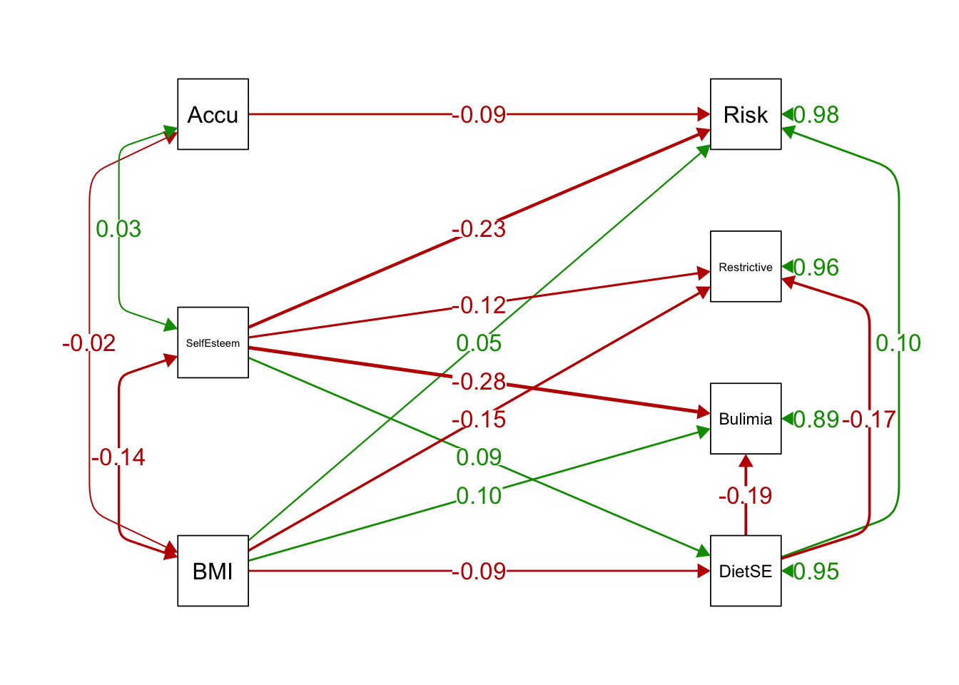
## 41 diff1 := med1-med4 diff1 0.034 0.008 4.243 0.000 0.020 0.051 0.034 0.034 0.0334.8.6 Plot it!
library(semPlot)

semPaths(ex5Boot, what='est',
         rotation = 2, # default rotation = 1 with four options
         curve = 2, # pull covariances' curves out a little
         nCharNodes = 0,
         nCharEdges = 0, # don't limit variable name lengths
         sizeMan = 8, # font size of manifest variable names
         style = "lisrel", # single-headed arrows vs. # "ram"'s 2-headed for variances
         edge.label.cex=1.2, curvePivot = TRUE,
         fade=FALSE)