Chapter 17 Lavaan Lab 14: Measurement Invariance
For this lab, we will run the MG-CFA analyses in class using simulated data based on Todd Little’s positive affect example.
Load up the lavaan library:
library(lavaan)and the dataset:
affectData <- read.csv("cfaInclassData.csv", header = T)For demonstration purposes, let’s first simulate a grouping variable called school:
set.seed(555)
affectData$school = sample(c('public', 'private'), nrow(affectData), replace = T)
table(affectData$school)
##
## private public
## 513 487head(affectData)## ID glad cheerful happy satisfied content comfortable school
## 1 1 0.13521092 0.5413297 -0.1041445 -0.5777446 0.8645383 0.02935020 private
## 2 2 -0.29116043 0.2434081 0.6671535 2.0763730 -0.7382832 1.05439183 public
## 3 3 0.71975913 0.2218277 0.4722337 2.1685984 -0.2727574 0.09053090 private
## 4 4 0.44432030 0.9295414 0.8574083 -1.0575363 -1.3841364 -0.07940091 private
## 5 5 2.84476524 3.1710123 3.5145040 1.5725274 2.3406754 1.59866763 public
## 6 6 -0.03317526 -0.8434011 -0.1485924 -0.5469343 -1.5750953 -0.69629828 publicThe goal of testing measurement invariance (MI) is to make sure that the scale that measures positive affect and satisfaction functions in the same way between public and private schools.
17.1 PART I: Multi-Group Analyses, Done Incorrectly
Syntax for an SR model (it doesn’t matter whether the model is for CFA or SR, the test of MI only applies to the CFA part):
srSyntax <- "
    posAffect =~ glad + happy + cheerful
    satisfaction =~ satisfied + content + comfortable

    # Structural Regression: beta
    satisfaction ~ posAffect
    "
MGsrRunWRONG <- lavaan::sem(srSyntax,
data = affectData,
fixed.x=FALSE,
group = "school", # group indicator
estimator = "MLR") # use MLR as a go-to estimation method
summary(MGsrRunWRONG, standardized = T, fit.measures = T)## lavaan 0.6-12 ended normally after 31 iterations
##
## Estimator ML
## Optimization method NLMINB
## Number of model parameters 38
##
## Number of observations per group:
## private 513
## public 487
##
## Model Test User Model:
## Standard Robust
## Test Statistic 11.920 11.709
## Degrees of freedom 16 16
## P-value (Chi-square) 0.749 0.764
## Scaling correction factor 1.018
## Yuan-Bentler correction (Mplus variant)
## Test statistic for each group:
## private 4.201 4.126
## public 7.719 7.583
##
## Model Test Baseline Model:
##
## Test statistic 2038.064 2039.295
## Degrees of freedom 30 30
## P-value 0.000 0.000
## Scaling correction factor 0.999
##
## User Model versus Baseline Model:
##
## Comparative Fit Index (CFI) 1.000 1.000
## Tucker-Lewis Index (TLI) 1.004 1.004
##
## Robust Comparative Fit Index (CFI) 1.000
## Robust Tucker-Lewis Index (TLI) 1.004
##
## Loglikelihood and Information Criteria:
##
## Loglikelihood user model (H0) -7473.002 -7473.002
## Scaling correction factor 1.001
## for the MLR correction
## Loglikelihood unrestricted model (H1) -7467.042 -7467.042
## Scaling correction factor 1.006
## for the MLR correction
##
## Akaike (AIC) 15022.004 15022.004
## Bayesian (BIC) 15208.498 15208.498
## Sample-size adjusted Bayesian (BIC) 15087.808 15087.808
##
## Root Mean Square Error of Approximation:
##
## RMSEA 0.000 0.000
## 90 Percent confidence interval - lower 0.000 0.000
## 90 Percent confidence interval - upper 0.030 0.029
## P-value RMSEA <= 0.05 0.998 0.999
##
## Robust RMSEA 0.000
## 90 Percent confidence interval - lower 0.000
## 90 Percent confidence interval - upper 0.029
##
## Standardized Root Mean Square Residual:
##
## SRMR 0.013 0.013
##
## Parameter Estimates:
##
## Standard errors Sandwich
## Information bread Observed
## Observed information based on Hessian
##
##
## Group 1 [private]:
##
## Latent Variables:
## Estimate Std.Err z-value P(>|z|) Std.lv Std.all
## posAffect =~
## glad 1.000 0.740 0.754
## happy 0.975 0.065 14.962 0.000 0.722 0.743
## cheerful 1.103 0.068 16.264 0.000 0.816 0.807
## satisfaction =~
## satisfied 1.000 0.792 0.779
## content 1.065 0.071 14.999 0.000 0.843 0.761
## comfortable 0.874 0.059 14.910 0.000 0.692 0.741
##
## Regressions:
## Estimate Std.Err z-value P(>|z|) Std.lv Std.all
## satisfaction ~
## posAffect 0.520 0.065 8.033 0.000 0.486 0.486
##
## Intercepts:
## Estimate Std.Err z-value P(>|z|) Std.lv Std.all
## .glad 0.023 0.043 0.530 0.596 0.023 0.023
## .happy 0.012 0.043 0.270 0.787 0.012 0.012
## .cheerful 0.027 0.045 0.594 0.553 0.027 0.026
## .satisfied -0.102 0.045 -2.269 0.023 -0.102 -0.100
## .content -0.086 0.049 -1.754 0.079 -0.086 -0.077
## .comfortable -0.061 0.041 -1.481 0.138 -0.061 -0.065
## posAffect 0.000 0.000 0.000
## .satisfaction 0.000 0.000 0.000
##
## Variances:
## Estimate Std.Err z-value P(>|z|) Std.lv Std.all
## .glad 0.417 0.037 11.257 0.000 0.417 0.432
## .happy 0.422 0.038 11.130 0.000 0.422 0.448
## .cheerful 0.357 0.037 9.643 0.000 0.357 0.349
## .satisfied 0.406 0.039 10.484 0.000 0.406 0.393
## .content 0.519 0.047 11.070 0.000 0.519 0.422
## .comfortable 0.393 0.036 10.765 0.000 0.393 0.451
## posAffect 0.548 0.059 9.213 0.000 1.000 1.000
## .satisfaction 0.478 0.057 8.380 0.000 0.763 0.763
##
##
## Group 2 [public]:
##
## Latent Variables:
## Estimate Std.Err z-value P(>|z|) Std.lv Std.all
## posAffect =~
## glad 1.000 0.643 0.655
## happy 1.182 0.091 13.041 0.000 0.761 0.775
## cheerful 1.130 0.091 12.455 0.000 0.727 0.764
## satisfaction =~
## satisfied 1.000 0.749 0.753
## content 1.072 0.072 14.806 0.000 0.803 0.763
## comfortable 0.972 0.065 14.904 0.000 0.729 0.753
##
## Regressions:
## Estimate Std.Err z-value P(>|z|) Std.lv Std.all
## satisfaction ~
## posAffect 0.568 0.074 7.725 0.000 0.488 0.488
##
## Intercepts:
## Estimate Std.Err z-value P(>|z|) Std.lv Std.all
## .glad -0.022 0.045 -0.492 0.623 -0.022 -0.022
## .happy 0.005 0.044 0.114 0.910 0.005 0.005
## .cheerful -0.030 0.043 -0.697 0.486 -0.030 -0.032
## .satisfied 0.018 0.045 0.399 0.690 0.018 0.018
## .content 0.012 0.048 0.251 0.802 0.012 0.011
## .comfortable -0.026 0.044 -0.597 0.551 -0.026 -0.027
## posAffect 0.000 0.000 0.000
## .satisfaction 0.000 0.000 0.000
##
## Variances:
## Estimate Std.Err z-value P(>|z|) Std.lv Std.all
## .glad 0.552 0.043 12.930 0.000 0.552 0.571
## .happy 0.385 0.043 8.958 0.000 0.385 0.400
## .cheerful 0.377 0.041 9.304 0.000 0.377 0.416
## .satisfied 0.429 0.042 10.338 0.000 0.429 0.433
## .content 0.462 0.048 9.576 0.000 0.462 0.417
## .comfortable 0.405 0.040 10.259 0.000 0.405 0.433
## posAffect 0.414 0.058 7.152 0.000 1.000 1.000
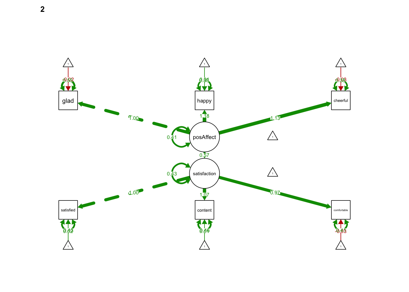
## .satisfaction 0.428 0.053 8.110 0.000 0.762 0.762library(semPlot)
semPaths(MGsrRunWRONG, what='est',
nCharNodes = 0,
nCharEdges = 0, # don't limit variable name lengths
edge.label.cex=0.6,
curvePivot = TRUE,
curve = 1.5, # pull covariances' curves out a little
fade=FALSE)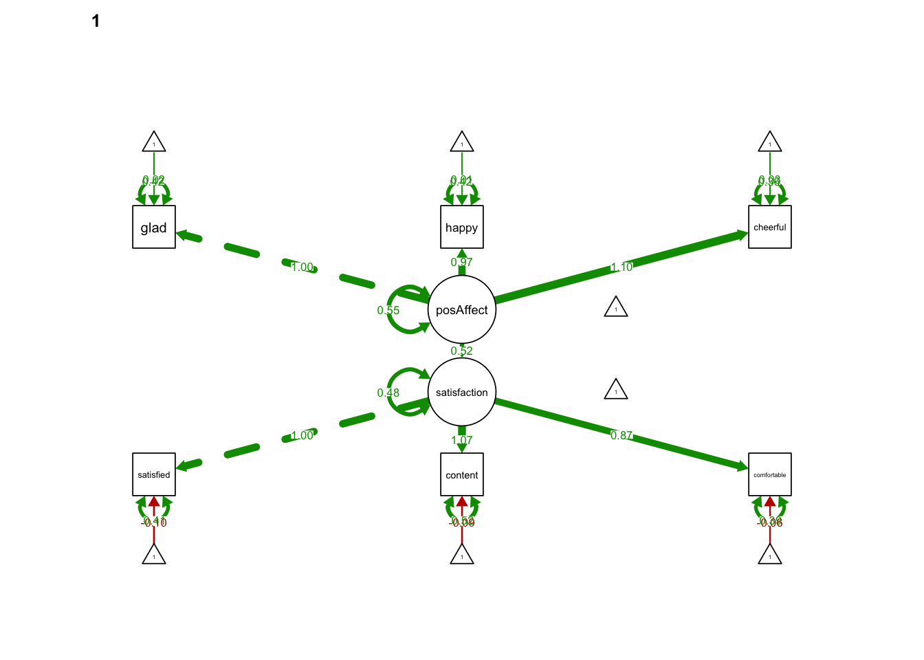
17.2 PART II: Testing Measurement Invariance
17.2.1 step 1: Configural invariance
If you simply use the MGsrRunWRONG synatx above, you are just testing configural invariance:
configuralFit <- lavaan::sem(srSyntax,
                    data = affectData,
                    fixed.x=FALSE,
                    group = "school", # group indicator
                    estimator = "MLR") # use MLR as a go-to estimation method
#summary(configuralFit, standardized = T, fit.measures = T)- Configural invariance was established due to satisfying model fit;
17.2.2 step 2: Metric (weak) invariance
To test metric invariance, you could manually constraint all factor loadings to be the same using tricks like “posAffect =~ c(lam1, lam1)*glad” but there is a shortcut using “group.equal” argument:
metricFit <- lavaan::sem(srSyntax,
                 data = affectData,
                 fixed.x=FALSE,
                 estimator = 'MLR',
                 group = "school",
group.equal = c("loadings")) - so that all factor loadings are fixed to be the same across groups
- More group equality constraints can be added, like “intercepts”, “means”, “residuals”, “residual.covariances”, “lv.variances”, “lv.covariances”, “regressions”
summary(metricFit, standardized = T, fit.measures = T)## lavaan 0.6-12 ended normally after 25 iterations
##
## Estimator ML
## Optimization method NLMINB
## Number of model parameters 38
## Number of equality constraints 4
##
## Number of observations per group:
## private 513
## public 487
##
## Model Test User Model:
## Standard Robust
## Test Statistic 17.640 17.639
## Degrees of freedom 20 20
## P-value (Chi-square) 0.611 0.611
## Scaling correction factor 1.000
## Yuan-Bentler correction (Mplus variant)
## Test statistic for each group:
## private 6.665 6.665
## public 10.975 10.974
##
## Model Test Baseline Model:
##
## Test statistic 2038.064 2039.295
## Degrees of freedom 30 30
## P-value 0.000 0.000
## Scaling correction factor 0.999
##
## User Model versus Baseline Model:
##
## Comparative Fit Index (CFI) 1.000 1.000
## Tucker-Lewis Index (TLI) 1.002 1.002
##
## Robust Comparative Fit Index (CFI) 1.000
## Robust Tucker-Lewis Index (TLI) 1.002
##
## Loglikelihood and Information Criteria:
##
## Loglikelihood user model (H0) -7475.862 -7475.862
## Scaling correction factor 0.904
## for the MLR correction
## Loglikelihood unrestricted model (H1) -7467.042 -7467.042
## Scaling correction factor 1.006
## for the MLR correction
##
## Akaike (AIC) 15019.724 15019.724
## Bayesian (BIC) 15186.588 15186.588
## Sample-size adjusted Bayesian (BIC) 15078.602 15078.602
##
## Root Mean Square Error of Approximation:
##
## RMSEA 0.000 0.000
## 90 Percent confidence interval - lower 0.000 0.000
## 90 Percent confidence interval - upper 0.033 0.033
## P-value RMSEA <= 0.05 0.998 0.998
##
## Robust RMSEA 0.000
## 90 Percent confidence interval - lower 0.000
## 90 Percent confidence interval - upper 0.033
##
## Standardized Root Mean Square Residual:
##
## SRMR 0.019 0.019
##
## Parameter Estimates:
##
## Standard errors Sandwich
## Information bread Observed
## Observed information based on Hessian
##
##
## Group 1 [private]:
##
## Latent Variables:
## Estimate Std.Err z-value P(>|z|) Std.lv Std.all
## posAffect =~
## glad 1.000 0.718 0.740
## happy (.p2.) 1.057 0.054 19.585 0.000 0.759 0.767
## cheerfl (.p3.) 1.113 0.055 20.393 0.000 0.799 0.796
## satisfaction =~
## satisfd 1.000 0.778 0.770
## content (.p5.) 1.069 0.051 21.078 0.000 0.832 0.754
## cmfrtbl (.p6.) 0.919 0.044 21.033 0.000 0.715 0.757
##
## Regressions:
## Estimate Std.Err z-value P(>|z|) Std.lv Std.all
## satisfaction ~
## posAffect 0.529 0.063 8.333 0.000 0.488 0.488
##
## Intercepts:
## Estimate Std.Err z-value P(>|z|) Std.lv Std.all
## .glad 0.023 0.043 0.530 0.596 0.023 0.024
## .happy 0.012 0.043 0.270 0.787 0.012 0.012
## .cheerful 0.027 0.045 0.594 0.553 0.027 0.026
## .satisfied -0.102 0.045 -2.269 0.023 -0.102 -0.101
## .content -0.086 0.049 -1.754 0.079 -0.086 -0.078
## .comfortable -0.061 0.041 -1.481 0.138 -0.061 -0.065
## posAffect 0.000 0.000 0.000
## .satisfaction 0.000 0.000 0.000
##
## Variances:
## Estimate Std.Err z-value P(>|z|) Std.lv Std.all
## .glad 0.427 0.036 11.943 0.000 0.427 0.453
## .happy 0.403 0.037 10.793 0.000 0.403 0.411
## .cheerful 0.370 0.035 10.705 0.000 0.370 0.367
## .satisfied 0.415 0.036 11.539 0.000 0.415 0.407
## .content 0.525 0.044 11.903 0.000 0.525 0.431
## .comfortable 0.381 0.035 10.927 0.000 0.381 0.427
## posAffect 0.516 0.053 9.799 0.000 1.000 1.000
## .satisfaction 0.461 0.051 9.082 0.000 0.762 0.762
##
##
## Group 2 [public]:
##
## Latent Variables:
## Estimate Std.Err z-value P(>|z|) Std.lv Std.all
## posAffect =~
## glad 1.000 0.673 0.675
## happy (.p2.) 1.057 0.054 19.585 0.000 0.711 0.740
## cheerfl (.p3.) 1.113 0.055 20.393 0.000 0.748 0.780
## satisfaction =~
## satisfd 1.000 0.763 0.761
## content (.p5.) 1.069 0.051 21.078 0.000 0.816 0.771
## cmfrtbl (.p6.) 0.919 0.044 21.033 0.000 0.701 0.734
##
## Regressions:
## Estimate Std.Err z-value P(>|z|) Std.lv Std.all
## satisfaction ~
## posAffect 0.557 0.067 8.342 0.000 0.492 0.492
##
## Intercepts:
## Estimate Std.Err z-value P(>|z|) Std.lv Std.all
## .glad -0.022 0.045 -0.492 0.623 -0.022 -0.022
## .happy 0.005 0.044 0.114 0.910 0.005 0.005
## .cheerful -0.030 0.043 -0.697 0.486 -0.030 -0.031
## .satisfied 0.018 0.045 0.399 0.690 0.018 0.018
## .content 0.012 0.048 0.251 0.802 0.012 0.011
## .comfortable -0.026 0.044 -0.597 0.551 -0.026 -0.027
## posAffect 0.000 0.000 0.000
## .satisfaction 0.000 0.000 0.000
##
## Variances:
## Estimate Std.Err z-value P(>|z|) Std.lv Std.all
## .glad 0.541 0.042 12.899 0.000 0.541 0.545
## .happy 0.418 0.040 10.351 0.000 0.418 0.452
## .cheerful 0.360 0.038 9.399 0.000 0.360 0.392
## .satisfied 0.423 0.040 10.551 0.000 0.423 0.421
## .content 0.454 0.045 10.053 0.000 0.454 0.406
## .comfortable 0.420 0.038 11.052 0.000 0.420 0.461
## posAffect 0.453 0.049 9.180 0.000 1.000 1.000
## .satisfaction 0.441 0.048 9.107 0.000 0.758 0.758- Again, metric invariance was established due to satisfying model fit;
- To test whether the equal factor loading assumption caused damage to model fit, we compare metricFit to configuralFit:
Model comparison:
anova(configuralFit, metricFit)## Scaled Chi-Squared Difference Test (method = "satorra.bentler.2001")
##
## lavaan NOTE:
## The "Chisq" column contains standard test statistics, not the
## robust test that should be reported per model. A robust difference
## test is a function of two standard (not robust) statistics.
##
## Df AIC BIC Chisq Chisq diff Df diff Pr(>Chisq)
## configuralFit 16 15022 15208 11.92
## metricFit 20 15020 15187 17.64 6.1624 4 0.1873- The test was not significant, meaning the increase in chi-square (due to the assumption of equal factor loadings) was not substantial enough to worsen the model fit;
- Note that this test suffers from the same problem as the chi-square test (too sensitive to model misfit)
17.2.3 step 3: Scalar (strong) Invariance
In this step, both factor loadings and measurement intercepts (of course, including factor structure) are constrained to be equal between the groups:
scalarFit <- lavaan::sem(srSyntax,
                 data = affectData,
                 fixed.x=FALSE,
                 estimator = 'MLR',
                 group = "school",
                 group.equal = c("loadings", "intercepts"))
summary(scalarFit, standardized = T, fit.measures = T)
## lavaan 0.6-12 ended normally after 32 iterations
##
## Estimator ML
## Optimization method NLMINB
## Number of model parameters 40
## Number of equality constraints 10
##
## Number of observations per group:
## private 513
## public 487
##
## Model Test User Model:
## Standard Robust
## Test Statistic 20.364 20.360
## Degrees of freedom 24 24
## P-value (Chi-square) 0.676 0.676
## Scaling correction factor 1.000
## Yuan-Bentler correction (Mplus variant)
## Test statistic for each group:
## private 7.764 7.762
## public 12.600 12.598
##
## Model Test Baseline Model:
##
## Test statistic 2038.064 2039.295
## Degrees of freedom 30 30
## P-value 0.000 0.000
## Scaling correction factor 0.999
##
## User Model versus Baseline Model:
##
## Comparative Fit Index (CFI) 1.000 1.000
## Tucker-Lewis Index (TLI) 1.002 1.002
##
## Robust Comparative Fit Index (CFI) 1.000
## Robust Tucker-Lewis Index (TLI) 1.002
##
## Loglikelihood and Information Criteria:
##
## Loglikelihood user model (H0) -7477.224 -7477.224
## Scaling correction factor 0.758
## for the MLR correction
## Loglikelihood unrestricted model (H1) -7467.042 -7467.042
## Scaling correction factor 1.006
## for the MLR correction
##
## Akaike (AIC) 15014.448 15014.448
## Bayesian (BIC) 15161.681 15161.681
## Sample-size adjusted Bayesian (BIC) 15066.399 15066.399
##
## Root Mean Square Error of Approximation:
##
## RMSEA 0.000 0.000
## 90 Percent confidence interval - lower 0.000 0.000
## 90 Percent confidence interval - upper 0.029 0.029
## P-value RMSEA <= 0.05 0.999 0.999
##
## Robust RMSEA 0.000
## 90 Percent confidence interval - lower 0.000
## 90 Percent confidence interval - upper 0.029
##
## Standardized Root Mean Square Residual:
##
## SRMR 0.020 0.020
##
## Parameter Estimates:
##
## Standard errors Sandwich
## Information bread Observed
## Observed information based on Hessian
##
##
## Group 1 [private]:
##
## Latent Variables:
## Estimate Std.Err z-value P(>|z|) Std.lv Std.all
## posAffect =~
## glad 1.000 0.718 0.740
## happy (.p2.) 1.056 0.054 19.522 0.000 0.759 0.767
## cheerfl (.p3.) 1.113 0.055 20.413 0.000 0.800 0.796
## satisfaction =~
## satisfd 1.000 0.780 0.771
## content (.p5.) 1.068 0.051 21.059 0.000 0.832 0.754
## cmfrtbl (.p6.) 0.915 0.043 21.140 0.000 0.713 0.755
##
## Regressions:
## Estimate Std.Err z-value P(>|z|) Std.lv Std.all
## satisfaction ~
## posAffect 0.530 0.063 8.350 0.000 0.488 0.488
##
## Intercepts:
## Estimate Std.Err z-value P(>|z|) Std.lv Std.all
## .glad (.16.) 0.019 0.040 0.462 0.644 0.019 0.019
## .happy (.17.) 0.026 0.040 0.644 0.519 0.026 0.026
## .cheerfl (.18.) 0.018 0.042 0.415 0.678 0.018 0.017
## .satisfd (.19.) -0.085 0.042 -2.031 0.042 -0.085 -0.084
## .content (.20.) -0.082 0.045 -1.820 0.069 -0.082 -0.075
## .cmfrtbl (.21.) -0.081 0.038 -2.108 0.035 -0.081 -0.086
## psAffct 0.000 0.000 0.000
## .stsfctn 0.000 0.000 0.000
##
## Variances:
## Estimate Std.Err z-value P(>|z|) Std.lv Std.all
## .glad 0.427 0.036 11.937 0.000 0.427 0.453
## .happy 0.403 0.037 10.809 0.000 0.403 0.412
## .cheerful 0.370 0.035 10.680 0.000 0.370 0.367
## .satisfied 0.414 0.036 11.505 0.000 0.414 0.405
## .content 0.525 0.044 11.872 0.000 0.525 0.431
## .comfortable 0.383 0.035 11.042 0.000 0.383 0.430
## posAffect 0.516 0.053 9.801 0.000 1.000 1.000
## .satisfaction 0.463 0.051 9.090 0.000 0.762 0.762
##
##
## Group 2 [public]:
##
## Latent Variables:
## Estimate Std.Err z-value P(>|z|) Std.lv Std.all
## posAffect =~
## glad 1.000 0.673 0.675
## happy (.p2.) 1.056 0.054 19.522 0.000 0.710 0.739
## cheerfl (.p3.) 1.113 0.055 20.413 0.000 0.749 0.780
## satisfaction =~
## satisfd 1.000 0.764 0.762
## content (.p5.) 1.068 0.051 21.059 0.000 0.816 0.771
## cmfrtbl (.p6.) 0.915 0.043 21.140 0.000 0.699 0.732
##
## Regressions:
## Estimate Std.Err z-value P(>|z|) Std.lv Std.all
## satisfaction ~
## posAffect 0.558 0.067 8.350 0.000 0.492 0.492
##
## Intercepts:
## Estimate Std.Err z-value P(>|z|) Std.lv Std.all
## .glad (.16.) 0.019 0.040 0.462 0.644 0.019 0.019
## .happy (.17.) 0.026 0.040 0.644 0.519 0.026 0.027
## .cheerfl (.18.) 0.018 0.042 0.415 0.678 0.018 0.018
## .satisfd (.19.) -0.085 0.042 -2.031 0.042 -0.085 -0.085
## .content (.20.) -0.082 0.045 -1.820 0.069 -0.082 -0.078
## .cmfrtbl (.21.) -0.081 0.038 -2.108 0.035 -0.081 -0.085
## psAffct -0.035 0.049 -0.697 0.486 -0.051 -0.051
## .stsfctn 0.104 0.051 2.053 0.040 0.137 0.137
##
## Variances:
## Estimate Std.Err z-value P(>|z|) Std.lv Std.all
## .glad 0.541 0.042 12.891 0.000 0.541 0.545
## .happy 0.419 0.041 10.332 0.000 0.419 0.453
## .cheerful 0.360 0.038 9.378 0.000 0.360 0.391
## .satisfied 0.422 0.040 10.516 0.000 0.422 0.420
## .content 0.454 0.045 10.032 0.000 0.454 0.405
## .comfortable 0.422 0.038 11.095 0.000 0.422 0.463
## posAffect 0.453 0.049 9.174 0.000 1.000 1.000
## .satisfaction 0.443 0.049 9.101 0.000 0.758 0.758Model comparison:
anova(metricFit, scalarFit)## Scaled Chi-Squared Difference Test (method = "satorra.bentler.2001")
##
## lavaan NOTE:
## The "Chisq" column contains standard test statistics, not the
## robust test that should be reported per model. A robust difference
## test is a function of two standard (not robust) statistics.
##
## Df AIC BIC Chisq Chisq diff Df diff Pr(>Chisq)
## metricFit 20 15020 15187 17.640
## scalarFit 24 15014 15162 20.364 2.7216 4 0.6054- The test was not significant, meaning the increase in chi-square (due to the assumption of equal measurement intercepts) was not substantial enough to worsen the model fit;
- Scalar invariance was established;
17.2.4 step 4: (Optional) Residual variance (strict) invariance
resVarFit <- lavaan::sem(srSyntax,
                 data = affectData,
                 fixed.x=FALSE,
                 estimator = 'MLR',
                 group = "school",
                 group.equal = c("loadings", "intercepts", "residuals"))
summary(resVarFit, standardized = T, fit.measures = T)
## lavaan 0.6-12 ended normally after 32 iterations
##
## Estimator ML
## Optimization method NLMINB
## Number of model parameters 40
## Number of equality constraints 16
##
## Number of observations per group:
## private 513
## public 487
##
## Model Test User Model:
## Standard Robust
## Test Statistic 26.885 26.947
## Degrees of freedom 30 30
## P-value (Chi-square) 0.629 0.626
## Scaling correction factor 0.998
## Yuan-Bentler correction (Mplus variant)
## Test statistic for each group:
## private 11.454 11.481
## public 15.430 15.466
##
## Model Test Baseline Model:
##
## Test statistic 2038.064 2039.295
## Degrees of freedom 30 30
## P-value 0.000 0.000
## Scaling correction factor 0.999
##
## User Model versus Baseline Model:
##
## Comparative Fit Index (CFI) 1.000 1.000
## Tucker-Lewis Index (TLI) 1.002 1.002
##
## Robust Comparative Fit Index (CFI) 1.000
## Robust Tucker-Lewis Index (TLI) 1.002
##
## Loglikelihood and Information Criteria:
##
## Loglikelihood user model (H0) -7480.484 -7480.484
## Scaling correction factor 0.610
## for the MLR correction
## Loglikelihood unrestricted model (H1) -7467.042 -7467.042
## Scaling correction factor 1.006
## for the MLR correction
##
## Akaike (AIC) 15008.968 15008.968
## Bayesian (BIC) 15126.754 15126.754
## Sample-size adjusted Bayesian (BIC) 15050.529 15050.529
##
## Root Mean Square Error of Approximation:
##
## RMSEA 0.000 0.000
## 90 Percent confidence interval - lower 0.000 0.000
## 90 Percent confidence interval - upper 0.029 0.029
## P-value RMSEA <= 0.05 1.000 1.000
##
## Robust RMSEA 0.000
## 90 Percent confidence interval - lower 0.000
## 90 Percent confidence interval - upper 0.029
##
## Standardized Root Mean Square Residual:
##
## SRMR 0.023 0.023
##
## Parameter Estimates:
##
## Standard errors Sandwich
## Information bread Observed
## Observed information based on Hessian
##
##
## Group 1 [private]:
##
## Latent Variables:
## Estimate Std.Err z-value P(>|z|) Std.lv Std.all
## posAffect =~
## glad 1.000 0.713 0.716
## happy (.p2.) 1.063 0.054 19.648 0.000 0.758 0.765
## cheerfl (.p3.) 1.114 0.055 20.246 0.000 0.794 0.794
## satisfaction =~
## satisfd 1.000 0.781 0.770
## content (.p5.) 1.068 0.051 21.048 0.000 0.833 0.766
## cmfrtbl (.p6.) 0.915 0.043 21.139 0.000 0.714 0.748
##
## Regressions:
## Estimate Std.Err z-value P(>|z|) Std.lv Std.all
## satisfaction ~
## posAffect 0.537 0.064 8.445 0.000 0.491 0.491
##
## Intercepts:
## Estimate Std.Err z-value P(>|z|) Std.lv Std.all
## .glad (.16.) 0.018 0.040 0.443 0.658 0.018 0.018
## .happy (.17.) 0.026 0.040 0.650 0.516 0.026 0.026
## .cheerfl (.18.) 0.018 0.042 0.415 0.678 0.018 0.018
## .satisfd (.19.) -0.085 0.042 -2.026 0.043 -0.085 -0.084
## .content (.20.) -0.083 0.045 -1.825 0.068 -0.083 -0.076
## .cmfrtbl (.21.) -0.082 0.038 -2.136 0.033 -0.082 -0.086
## psAffct 0.000 0.000 0.000
## .stsfctn 0.000 0.000 0.000
##
## Variances:
## Estimate Std.Err z-value P(>|z|) Std.lv Std.all
## .glad (.p8.) 0.483 0.028 17.136 0.000 0.483 0.487
## .happy (.p9.) 0.408 0.029 14.229 0.000 0.408 0.415
## .cheerfl (.10.) 0.369 0.028 13.197 0.000 0.369 0.369
## .satisfd (.11.) 0.417 0.028 14.667 0.000 0.417 0.406
## .content (.12.) 0.490 0.034 14.545 0.000 0.490 0.414
## .cmfrtbl (.13.) 0.402 0.027 15.048 0.000 0.402 0.441
## psAffct 0.509 0.051 9.913 0.000 1.000 1.000
## .stsfctn 0.463 0.050 9.171 0.000 0.759 0.759
##
##
## Group 2 [public]:
##
## Latent Variables:
## Estimate Std.Err z-value P(>|z|) Std.lv Std.all
## posAffect =~
## glad 1.000 0.673 0.696
## happy (.p2.) 1.063 0.054 19.648 0.000 0.716 0.746
## cheerfl (.p3.) 1.114 0.055 20.246 0.000 0.750 0.777
## satisfaction =~
## satisfd 1.000 0.764 0.764
## content (.p5.) 1.068 0.051 21.048 0.000 0.816 0.759
## cmfrtbl (.p6.) 0.915 0.043 21.139 0.000 0.699 0.741
##
## Regressions:
## Estimate Std.Err z-value P(>|z|) Std.lv Std.all
## satisfaction ~
## posAffect 0.556 0.067 8.327 0.000 0.490 0.490
##
## Intercepts:
## Estimate Std.Err z-value P(>|z|) Std.lv Std.all
## .glad (.16.) 0.018 0.040 0.443 0.658 0.018 0.018
## .happy (.17.) 0.026 0.040 0.650 0.516 0.026 0.027
## .cheerfl (.18.) 0.018 0.042 0.415 0.678 0.018 0.018
## .satisfd (.19.) -0.085 0.042 -2.026 0.043 -0.085 -0.085
## .content (.20.) -0.083 0.045 -1.825 0.068 -0.083 -0.077
## .cmfrtbl (.21.) -0.082 0.038 -2.136 0.033 -0.082 -0.087
## psAffct -0.034 0.049 -0.693 0.488 -0.051 -0.051
## .stsfctn 0.104 0.051 2.049 0.040 0.136 0.136
##
## Variances:
## Estimate Std.Err z-value P(>|z|) Std.lv Std.all
## .glad (.p8.) 0.483 0.028 17.136 0.000 0.483 0.516
## .happy (.p9.) 0.408 0.029 14.229 0.000 0.408 0.443
## .cheerfl (.10.) 0.369 0.028 13.197 0.000 0.369 0.396
## .satisfd (.11.) 0.417 0.028 14.667 0.000 0.417 0.417
## .content (.12.) 0.490 0.034 14.545 0.000 0.490 0.424
## .cmfrtbl (.13.) 0.402 0.027 15.048 0.000 0.402 0.451
## psAffct 0.454 0.050 9.153 0.000 1.000 1.000
## .stsfctn 0.444 0.049 9.141 0.000 0.760 0.760Model comparison:
anova(resVarFit, scalarFit)## Scaled Chi-Squared Difference Test (method = "satorra.bentler.2001")
##
## lavaan NOTE:
## The "Chisq" column contains standard test statistics, not the
## robust test that should be reported per model. A robust difference
## test is a function of two standard (not robust) statistics.
##
## Df AIC BIC Chisq Chisq diff Df diff Pr(>Chisq)
## scalarFit 24 15014 15162 20.364
## resVarFit 30 15009 15127 26.885 6.6022 6 0.3592- The test was not significant, meaning the increase in chi-square (due to the assumption of equal residual variances) was not substantial enough to worsen the model fit;
- Strict invariance was established.
17.3 PART III: Shortcut to performing MI
17.3.1 measurementInvariance()
There is a shortcut function in package ‘semTools’ that performs invariance testing in one place, but unfortunately it will soon retire…
library(semTools)

measurementInvariance(model = srSyntax,
                      data = affectData,
                      fixed.x=FALSE,
                      estimator = 'MLR',
                      group = "school")
## Warning: The measurementInvariance function is deprecated, and it will cease to be included in future versions of semTools. See help('semTools-deprecated) for details.##
## Measurement invariance models:
##
## Model 1 : fit.configural
## Model 2 : fit.loadings
## Model 3 : fit.intercepts
## Model 4 : fit.means
##
## Scaled Chi-Squared Difference Test (method = "satorra.bentler.2001")
##
## lavaan NOTE:
## The "Chisq" column contains standard test statistics, not the
## robust test that should be reported per model. A robust difference
## test is a function of two standard (not robust) statistics.
##
## Df AIC BIC Chisq Chisq diff Df diff Pr(>Chisq)
## fit.configural 16 15022 15208 11.920
## fit.loadings 20 15020 15187 17.640 6.1624 4 0.1873
## fit.intercepts 24 15014 15162 20.364 2.7216 4 0.6054
## fit.means 26 15015 15152 24.826 4.4961 2 0.1056
##
##
## Fit measures:
##
## cfi.scaled rmsea.scaled cfi.scaled.delta rmsea.scaled.delta
## fit.configural 1 0 NA NA
## fit.loadings 1 0 0 0
## fit.intercepts 1 0 0 0
## fit.means 1 0 0 017.3.2 measEq.syntax()
To use measEq.syntax() from semTools, we need to use a model syntax for CFA model instead of SR model:
cfaSyntax <- "
    posAffect =~ glad + happy + cheerful
    satisfaction =~ satisfied + content + comfortable
    "
test.seq <- list(weak = c("loadings"),
strong = c("intercepts"),
strict = c("residuals"))
meq.list <- list()
for (i in 0:length(test.seq)) {
if (i == 0L) {
meq.label <- "configural"
group.equal <- ""
} else {
meq.label <- names(test.seq)[i]
group.equal <- unlist(test.seq[1:i])
}
meq.list[[meq.label]] <- measEq.syntax(configural.model = cfaSyntax,
data = affectData,
fixed.x = TRUE,
estimator = 'MLR',
group = "school",
group.equal = group.equal,
return.fit = TRUE)
}summary(compareFit(meq.list))## ################### Nested Model Comparison #########################
## Scaled Chi-Squared Difference Test (method = "satorra.bentler.2001")
##
## lavaan NOTE:
## The "Chisq" column contains standard test statistics, not the
## robust test that should be reported per model. A robust difference
## test is a function of two standard (not robust) statistics.
##
## Df AIC BIC Chisq Chisq diff Df diff Pr(>Chisq)
## meq.list.configural 16 15022 15208 11.920
## meq.list.weak 20 15020 15187 17.640 6.1624 4 0.1873
## meq.list.strong 24 15014 15162 20.364 2.7216 4 0.6054
## meq.list.strict 30 15009 15127 26.885 6.6022 6 0.3592
##
## ####################### Model Fit Indices ###########################
## chisq.scaled df.scaled pvalue.scaled rmsea.robust cfi.robust tli.robust srmr aic bic
## meq.list.configural 11.709† 16 .764 .000† 1.000† 1.004† .013† 15022.004 15208.498
## meq.list.weak 17.639 20 .611 .000† 1.000† 1.002 .019 15019.724 15186.588
## meq.list.strong 20.360 24 .676 .000† 1.000† 1.002 .020 15014.448 15161.681
## meq.list.strict 26.947 30 .626 .000† 1.000† 1.002 .023 15008.968† 15126.754†
##
## ################## Differences in Fit Indices #######################
## df.scaled rmsea.robust cfi.robust tli.robust srmr aic bic
## meq.list.weak - meq.list.configural 4 0 0 -0.002 0.006 -2.280 -21.911
## meq.list.strong - meq.list.weak 4 0 0 0.001 0.001 -5.276 -24.907
## meq.list.strict - meq.list.strong 6 0 0 -0.001 0.003 -5.480 -34.926According to Putnick & Bornstein (2016):
- Some researchers have shifted from a focus on absolute fit in terms of \(\chi^2\) to a focus on alternative fit indices because \(\chi^2\) is overly sensitive to small, unimportant deviations from a “perfect” model in large samples (Chen, 2007; Cheung & Rensvold, 2002; French & Finch, 2006; Meade, Johnson, & Braddy, 2008).
- Cheung and Rensvold’s (2002) criterion of a -.01 change in CFI for nested models is commonly used, but other researchers have suggested different criteria for CFI (Meade et al., 2008; Rutkowski & Svetina, 2014).
- This means in the last section of “Differences in Fit Indices”, a positive ‘cfi.robust’ or a negative ‘cfi.robust’>= -.01 helps establish measurement noninvariance.
17.4 PART IV: Multi-Group CFA Modeling, done right
- To compare the structural model parameters, at least scalar (strong) invariance is required;
- Since strict invariance was also satisfied, we will use resVarFit for MG-SR Modeling in this example:
17.4.1 Statistical Test of Equal Factor Means:
equalMeanfit <- lavaan::sem(cfaSyntax,
                    affectData,
                    fixed.x = FALSE,
                    estimator = 'MLR',
                    group = "school",
                    group.equal = c("loadings", "intercepts", "residuals",
                                    "means"))

summary(equalMeanfit, standardized = T, fit.measures = T)
## lavaan 0.6-12 ended normally after 28 iterations
##
## Estimator ML
## Optimization method NLMINB
## Number of model parameters 38
## Number of equality constraints 16
##
## Number of observations per group:
## private 513
## public 487
##
## Model Test User Model:
## Standard Robust
## Test Statistic 31.333 31.415
## Degrees of freedom 32 32
## P-value (Chi-square) 0.500 0.496
## Scaling correction factor 0.997
## Yuan-Bentler correction (Mplus variant)
## Test statistic for each group:
## private 13.747 13.784
## public 17.585 17.632
##
## Model Test Baseline Model:
##
## Test statistic 2038.064 2039.295
## Degrees of freedom 30 30
## P-value 0.000 0.000
## Scaling correction factor 0.999
##
## User Model versus Baseline Model:
##
## Comparative Fit Index (CFI) 1.000 1.000
## Tucker-Lewis Index (TLI) 1.000 1.000
##
## Robust Comparative Fit Index (CFI) 1.000
## Robust Tucker-Lewis Index (TLI) 1.000
##
## Loglikelihood and Information Criteria:
##
## Loglikelihood user model (H0) -7482.708 -7482.708
## Scaling correction factor 0.590
## for the MLR correction
## Loglikelihood unrestricted model (H1) -7467.042 -7467.042
## Scaling correction factor 1.006
## for the MLR correction
##
## Akaike (AIC) 15009.416 15009.416
## Bayesian (BIC) 15117.387 15117.387
## Sample-size adjusted Bayesian (BIC) 15047.514 15047.514
##
## Root Mean Square Error of Approximation:
##
## RMSEA 0.000 0.000
## 90 Percent confidence interval - lower 0.000 0.000
## 90 Percent confidence interval - upper 0.032 0.032
## P-value RMSEA <= 0.05 1.000 1.000
##
## Robust RMSEA 0.000
## 90 Percent confidence interval - lower 0.000
## 90 Percent confidence interval - upper 0.032
##
## Standardized Root Mean Square Residual:
##
## SRMR 0.028 0.028
##
## Parameter Estimates:
##
## Standard errors Sandwich
## Information bread Observed
## Observed information based on Hessian
##
##
## Group 1 [private]:
##
## Latent Variables:
## Estimate Std.Err z-value P(>|z|) Std.lv Std.all
## posAffect =~
## glad 1.000 0.713 0.716
## happy (.p2.) 1.064 0.054 19.659 0.000 0.759 0.766
## cheerfl (.p3.) 1.113 0.055 20.234 0.000 0.794 0.794
## satisfaction =~
## satisfd 1.000 0.781 0.770
## content (.p5.) 1.069 0.051 21.128 0.000 0.834 0.766
## cmfrtbl (.p6.) 0.917 0.043 21.128 0.000 0.716 0.749
##
## Covariances:
## Estimate Std.Err z-value P(>|z|) Std.lv Std.all
## posAffect ~~
## satisfaction 0.272 0.038 7.166 0.000 0.489 0.489
##
## Intercepts:
## Estimate Std.Err z-value P(>|z|) Std.lv Std.all
## .glad (.16.) 0.000 0.031 0.007 0.994 0.000 0.000
## .happy (.17.) 0.007 0.031 0.241 0.810 0.007 0.008
## .cheerfl (.18.) -0.002 0.031 -0.065 0.948 -0.002 -0.002
## .satisfd (.19.) -0.043 0.032 -1.360 0.174 -0.043 -0.043
## .content (.20.) -0.038 0.034 -1.111 0.267 -0.038 -0.035
## .cmfrtbl (.21.) -0.044 0.030 -1.459 0.144 -0.044 -0.046
## psAffct 0.000 0.000 0.000
## stsfctn 0.000 0.000 0.000
##
## Variances:
## Estimate Std.Err z-value P(>|z|) Std.lv Std.all
## .glad (.p7.) 0.484 0.028 17.125 0.000 0.484 0.487
## .happy (.p8.) 0.407 0.029 14.219 0.000 0.407 0.414
## .cheerfl (.p9.) 0.369 0.028 13.207 0.000 0.369 0.369
## .satisfd (.10.) 0.419 0.028 14.741 0.000 0.419 0.407
## .content (.11.) 0.491 0.034 14.588 0.000 0.491 0.413
## .cmfrtbl (.12.) 0.401 0.027 14.918 0.000 0.401 0.439
## psAffct 0.509 0.051 9.894 0.000 1.000 1.000
## stsfctn 0.609 0.064 9.549 0.000 1.000 1.000
##
##
## Group 2 [public]:
##
## Latent Variables:
## Estimate Std.Err z-value P(>|z|) Std.lv Std.all
## posAffect =~
## glad 1.000 0.674 0.696
## happy (.p2.) 1.064 0.054 19.659 0.000 0.717 0.747
## cheerfl (.p3.) 1.113 0.055 20.234 0.000 0.750 0.777
## satisfaction =~
## satisfd 1.000 0.765 0.763
## content (.p5.) 1.069 0.051 21.128 0.000 0.817 0.759
## cmfrtbl (.p6.) 0.917 0.043 21.128 0.000 0.701 0.742
##
## Covariances:
## Estimate Std.Err z-value P(>|z|) Std.lv Std.all
## posAffect ~~
## satisfaction 0.251 0.035 7.161 0.000 0.488 0.488
##
## Intercepts:
## Estimate Std.Err z-value P(>|z|) Std.lv Std.all
## .glad (.16.) 0.000 0.031 0.007 0.994 0.000 0.000
## .happy (.17.) 0.007 0.031 0.241 0.810 0.007 0.008
## .cheerfl (.18.) -0.002 0.031 -0.065 0.948 -0.002 -0.002
## .satisfd (.19.) -0.043 0.032 -1.360 0.174 -0.043 -0.043
## .content (.20.) -0.038 0.034 -1.111 0.267 -0.038 -0.035
## .cmfrtbl (.21.) -0.044 0.030 -1.459 0.144 -0.044 -0.046
## psAffct 0.000 0.000 0.000
## stsfctn 0.000 0.000 0.000
##
## Variances:
## Estimate Std.Err z-value P(>|z|) Std.lv Std.all
## .glad (.p7.) 0.484 0.028 17.125 0.000 0.484 0.516
## .happy (.p8.) 0.407 0.029 14.219 0.000 0.407 0.442
## .cheerfl (.p9.) 0.369 0.028 13.207 0.000 0.369 0.396
## .satisfd (.10.) 0.419 0.028 14.741 0.000 0.419 0.417
## .content (.11.) 0.491 0.034 14.588 0.000 0.491 0.424
## .cmfrtbl (.12.) 0.401 0.027 14.918 0.000 0.401 0.449
## psAffct 0.454 0.050 9.164 0.000 1.000 1.000
## stsfctn 0.585 0.057 10.290 0.000 1.000 1.000anova(resVarFit, equalMeanfit)## Scaled Chi-Squared Difference Test (method = "satorra.bentler.2001")
##
## lavaan NOTE:
## The "Chisq" column contains standard test statistics, not the
## robust test that should be reported per model. A robust difference
## test is a function of two standard (not robust) statistics.
##
## Df AIC BIC Chisq Chisq diff Df diff Pr(>Chisq)
## resVarFit 30 15009 15127 26.885
## equalMeanfit 32 15009 15117 31.333 4.4815 2 0.1064- The anova test was not significant, meaning the increase in chi-square (due to the constraint of equal latent means) was not substantial enough to worsen the model fit;
- It says the levels of positive affect and satisfaction in public schools were essentially the same as those in private schools.
17.4.2 Statistical Test of Equal Regression Coefficients:
- Note that we used srSyntax here because we need to define the regression coefficient between PA and satisfaction:
equalBetafit <- lavaan::sem(srSyntax,
                    affectData,
                    fixed.x = FALSE,
                    estimator = 'MLR',
                    group = "school",
                    group.equal = c("loadings", "intercepts", "residuals",
                                 "regressions"))

summary(equalBetafit, standardized = T, fit.measures = T)
## lavaan 0.6-12 ended normally after 30 iterations
##
## Estimator ML
## Optimization method NLMINB
## Number of model parameters 40
## Number of equality constraints 17
##
## Number of observations per group:
## private 513
## public 487
##
## Model Test User Model:
## Standard Robust
## Test Statistic 26.937 26.888
## Degrees of freedom 31 31
## P-value (Chi-square) 0.675 0.678
## Scaling correction factor 1.002
## Yuan-Bentler correction (Mplus variant)
## Test statistic for each group:
## private 11.496 11.476
## public 15.441 15.413
##
## Model Test Baseline Model:
##
## Test statistic 2038.064 2039.295
## Degrees of freedom 30 30
## P-value 0.000 0.000
## Scaling correction factor 0.999
##
## User Model versus Baseline Model:
##
## Comparative Fit Index (CFI) 1.000 1.000
## Tucker-Lewis Index (TLI) 1.002 1.002
##
## Robust Comparative Fit Index (CFI) 1.000
## Robust Tucker-Lewis Index (TLI) 1.002
##
## Loglikelihood and Information Criteria:
##
## Loglikelihood user model (H0) -7480.510 -7480.510
## Scaling correction factor 0.582
## for the MLR correction
## Loglikelihood unrestricted model (H1) -7467.042 -7467.042
## Scaling correction factor 1.006
## for the MLR correction
##
## Akaike (AIC) 15007.021 15007.021
## Bayesian (BIC) 15119.899 15119.899
## Sample-size adjusted Bayesian (BIC) 15046.850 15046.850
##
## Root Mean Square Error of Approximation:
##
## RMSEA 0.000 0.000
## 90 Percent confidence interval - lower 0.000 0.000
## 90 Percent confidence interval - upper 0.027 0.027
## P-value RMSEA <= 0.05 1.000 1.000
##
## Robust RMSEA 0.000
## 90 Percent confidence interval - lower 0.000
## 90 Percent confidence interval - upper 0.027
##
## Standardized Root Mean Square Residual:
##
## SRMR 0.024 0.024
##
## Parameter Estimates:
##
## Standard errors Sandwich
## Information bread Observed
## Observed information based on Hessian
##
##
## Group 1 [private]:
##
## Latent Variables:
## Estimate Std.Err z-value P(>|z|) Std.lv Std.all
## posAffect =~
## glad 1.000 0.712 0.716
## happy (.p2.) 1.064 0.054 19.668 0.000 0.758 0.765
## cheerfl (.p3.) 1.114 0.055 20.253 0.000 0.794 0.794
## satisfaction =~
## satisfd 1.000 0.783 0.771
## content (.p5.) 1.067 0.051 21.045 0.000 0.836 0.767
## cmfrtbl (.p6.) 0.915 0.043 21.157 0.000 0.716 0.749
##
## Regressions:
## Estimate Std.Err z-value P(>|z|) Std.lv Std.all
## satisfaction ~
## psAffct (.p7.) 0.546 0.048 11.266 0.000 0.497 0.497
##
## Intercepts:
## Estimate Std.Err z-value P(>|z|) Std.lv Std.all
## .glad (.16.) 0.018 0.040 0.443 0.658 0.018 0.018
## .happy (.17.) 0.026 0.040 0.650 0.516 0.026 0.026
## .cheerfl (.18.) 0.018 0.042 0.415 0.678 0.018 0.018
## .satisfd (.19.) -0.085 0.042 -2.026 0.043 -0.085 -0.084
## .content (.20.) -0.083 0.045 -1.825 0.068 -0.083 -0.076
## .cmfrtbl (.21.) -0.082 0.038 -2.137 0.033 -0.082 -0.086
## psAffct 0.000 0.000 0.000
## .stsfctn 0.000 0.000 0.000
##
## Variances:
## Estimate Std.Err z-value P(>|z|) Std.lv Std.all
## .glad (.p8.) 0.483 0.028 17.135 0.000 0.483 0.488
## .happy (.p9.) 0.407 0.029 14.260 0.000 0.407 0.415
## .cheerfl (.10.) 0.369 0.028 13.259 0.000 0.369 0.370
## .satisfd (.11.) 0.417 0.028 14.675 0.000 0.417 0.405
## .content (.12.) 0.490 0.034 14.542 0.000 0.490 0.412
## .cmfrtbl (.13.) 0.402 0.027 15.067 0.000 0.402 0.439
## psAffct 0.508 0.051 9.911 0.000 1.000 1.000
## .stsfctn 0.462 0.050 9.171 0.000 0.753 0.753
##
##
## Group 2 [public]:
##
## Latent Variables:
## Estimate Std.Err z-value P(>|z|) Std.lv Std.all
## posAffect =~
## glad 1.000 0.674 0.696
## happy (.p2.) 1.064 0.054 19.668 0.000 0.717 0.747
## cheerfl (.p3.) 1.114 0.055 20.253 0.000 0.751 0.777
## satisfaction =~
## satisfd 1.000 0.762 0.763
## content (.p5.) 1.067 0.051 21.045 0.000 0.813 0.758
## cmfrtbl (.p6.) 0.915 0.043 21.157 0.000 0.697 0.740
##
## Regressions:
## Estimate Std.Err z-value P(>|z|) Std.lv Std.all
## satisfaction ~
## psAffct (.p7.) 0.546 0.048 11.266 0.000 0.483 0.483
##
## Intercepts:
## Estimate Std.Err z-value P(>|z|) Std.lv Std.all
## .glad (.16.) 0.018 0.040 0.443 0.658 0.018 0.018
## .happy (.17.) 0.026 0.040 0.650 0.516 0.026 0.027
## .cheerfl (.18.) 0.018 0.042 0.415 0.678 0.018 0.018
## .satisfd (.19.) -0.085 0.042 -2.026 0.043 -0.085 -0.085
## .content (.20.) -0.083 0.045 -1.825 0.068 -0.083 -0.077
## .cmfrtbl (.21.) -0.082 0.038 -2.137 0.033 -0.082 -0.087
## psAffct -0.034 0.049 -0.693 0.488 -0.051 -0.051
## .stsfctn 0.104 0.051 2.046 0.041 0.136 0.136
##
## Variances:
## Estimate Std.Err z-value P(>|z|) Std.lv Std.all
## .glad (.p8.) 0.483 0.028 17.135 0.000 0.483 0.515
## .happy (.p9.) 0.407 0.029 14.260 0.000 0.407 0.442
## .cheerfl (.10.) 0.369 0.028 13.259 0.000 0.369 0.396
## .satisfd (.11.) 0.417 0.028 14.675 0.000 0.417 0.418
## .content (.12.) 0.490 0.034 14.542 0.000 0.490 0.426
## .cmfrtbl (.13.) 0.402 0.027 15.067 0.000 0.402 0.453
## psAffct 0.454 0.049 9.228 0.000 1.000 1.000
## .stsfctn 0.445 0.048 9.293 0.000 0.767 0.767anova(resVarFit, equalBetafit)## Scaled Chi-Squared Difference Test (method = "satorra.bentler.2001")
##
## lavaan NOTE:
## The "Chisq" column contains standard test statistics, not the
## robust test that should be reported per model. A robust difference
## test is a function of two standard (not robust) statistics.
##
## Df AIC BIC Chisq Chisq diff Df diff Pr(>Chisq)
## resVarFit 30 15009 15127 26.885
## equalBetafit 31 15007 15120 26.937 0.046657 1 0.829- The test was not significant, meaning the increase in chi-square (due to the constraint of equal regression coefficients) was not substantial enough to worsen the model fit;
- It says the effect of positive affect on satisfaction in public schools was essentially the same as that in private schools.